There’s a nice new article on Wynne Godley today in The New York Times.
An interesting thing in the article is the mention of intuition via models while mentioning his book Monetary Economics.
Why does a model matter? It explicitly details an economist’s thinking, Dr. Bezemer says. Other economists can use it. They cannot so easily clone intuition.
That is so right. The models in the books of Wynne Godley – both Monetary Economics with Marc Lavoie and Macroeconomics with Francis Cripps give a good idea about the authors’ intuitions. Of course, needless to say the man was bigger than his models.
Over this thread at Matias Vernengo’s blog Naked Keynesianism, I got into an exchange about current account deficits and sustainability with an anonymous commenter – a topic I had blogged on recently in 2-3 posts.
The commenter seems to not understand how this works or seems to believe that net indebtedness cannot keep rising relative to GDP in scenarios. I will present some scenarios below. The scenario presented below is not what literally happens but rather shows the absurdity of some types of growth.
Before this, let me give the expression for net indebtedness to foreigners. Ignoring revaluations, only current account transactions change claims on foreigners or claims by foreigners on residents. So
Change in Net Indebtedness to Foreigners = Current Account Deficit.
For simplicity, I will ignore other items in the current account – such as interest and dividend payments between residents and non-residents etc.
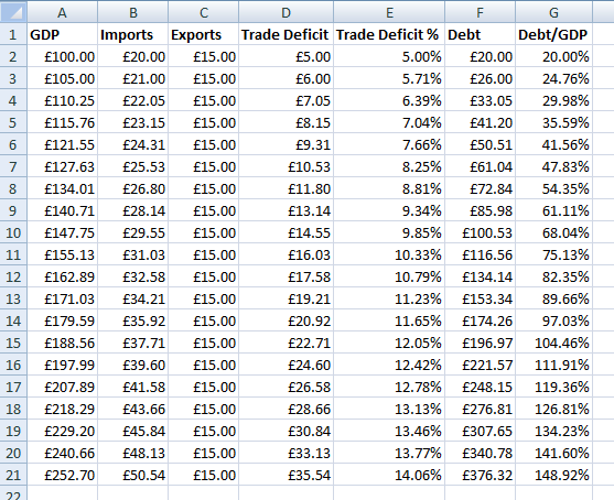
So start with GDP of £100, imports of £20 and exports of £15 and net indebtedness to foreigners of 20% of GDP.
Assume GDP grows at 5% annually. Imports as a percent of GDP is 20% and exports do not grow.
(In real life imports can be even worse when output changes but let’s just keep things simpler).
The numbers are nominal values.
So here is how it looks in Excel:
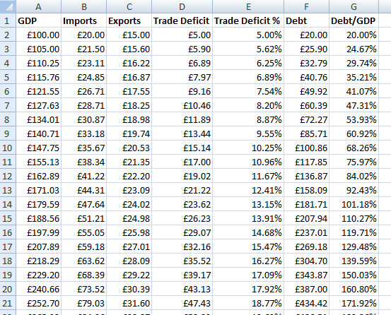
Now one can argue about the simplicity in the assumption that export was held constant. So here it is at 4% export growth.
To make it more realistic, I also use import elasticity of 1.5 – which means that for a 1% rise in GDP, imports rise by 1.5%.
Deteriorating in either case. If you were to extend the scenario to more rows in Excel, you can see how it rises forever.
It illustrates one thing: At sufficiently low growth of exports or a high propensity to import, a faster rate of growth of output comes with net indebtedness to foreigners rising relative to GDP which cannot be sustained for long.
Also if one assumes (although not always the case) that the private sector net accumulation of financial assets (NAFA) is a small positive number (such as 2% of GDP), then the current account reflects directly on the fiscal deficit because of the sectoral balances identity.
You can do this on your own sheet and see how these numbers change for different scenarios assumed.
The reason I have a numerical example is that it is easier to see how fast these stocks and flows change.
This example is an illustration of the balance-of-payments constraint nations face. Faced with rising current account imbalances, nations may be faced with little optimism – such as the ability to use of fiscal policy to improve demand and output. In a world of free trade, there is less one can do such as raising tariffs, import controls and so on. The trend in international political economy is actually tending toward reducing tariffs which makes the problem even worse. Subsidies to exporters can be provided but these lead to cries of foul at WTO. Even if subsidies are given to exporters, they are limited by how well they can compete with big firms in international markets. When this happens for everyone – such as at present – an international political economy game happens where muddled policy makers try to discuss something but in the end vow to continue free trade policies. Or they play games such as beggar-my-neighbour. Whatever said, a nation’s success crucially depends on how their producers do in international markets.
Back to stocks and flows. In real life things get more complicated and interesting. A nation may receive a lot of payments from abroad – even if its trade balance is worsening because of direct investments made in the past etc. Residents hold stock market securities abroad and these may make a killing – so analysing this becomes even more interesting! So high holding gains of assets held abroad may be sufficient to prevent net indebtedness from rising even if the current account balance is high. So there is an interesting dynamics here but finally, the current account balance wins over revaluations.
The example is motivated by one given in Wynne Godley and Francis Cripps’ book Macroeconomics.
I like Steve Keen. He is terrific in debunking economics! In a recent debate with Paul Krugman, Keen put Krugman on the defensive and exposed his weaknesses. Krugman obviously didn’t want to accept defeat and tried to escape with the help of comments in the comments section of Nick Rowe’s blog (that DSGE is not neoclassical – whatever!).
There are however some issues with Keen’s own methodologies. In a recent talk (video here), he claims that income is not equal to expenditure due to debt creation. Keen also claims in the video that Schumpeter and Minsky claimed that is the case.
Keen is right about an individual sector but not an economy as a whole when it is closed.
In the following I assume a closed economy – as does Keen. At least he doesn’t make any distinction and thereby his claim is a claim for a closed economy as well. So here is Keen’s claim:
Further he attributes this difference to discontinuities due to debt injections.
In the above Keen forgets that expenditure creates income.
There is no need for a claim that income is not equal to expenditure. In fact it is convenient to have them equal.
Wynne Godley and Francis Cripps wrote a nice book in 1983 named Macroeconomics. Here is from just the second page of Chapter 1: National Accounts:
It is extremely useful to choose definitions such that total income and expenditure in any year, month, day or second are identically equal to one another; they will be – because we choose to define them so that they are – two different ways of looking at the same process. We are only going to admit into the category of flows called income things which have an exact counterpart in the category of flows called expenditure. [footnote]
(with a footnote on qualifications for the case of an open economy).
Further in pages 27-29:
Although the definitions so far imply that the income of all individuals and institutions taken together equals their total expenditure on goods and services in each and every period, this need not be true of any particular person or institution …
… It is easy to understand that any one individual who does not spend all his or her income in a period will have more money left over at the end of the period. But we have chosen a system of definitions which ensures that total income in each period when summed across the whole economy equals total expenditure in the same period. It must therefore be the case that if some people or institutions are accumulating money or other financial assets, others are incurring debts on an exactly equal scale. In the economy as a whole the total increase in financial assets must always be equal in each period to the total increase in debt (financial liabilities).
But since the possibility of borrowing is included as a source of funds for spending, our formal representation of the budget constraint for any individual or institution including the government, is
Equation 1.4 simply says that any excess of income over spending must equal the acquisition of financial assets less the acquisition of debts. As this is true for all individuals it must also be true for the economy as a whole.
But since total national income equals total national expenditure (i.e., Y ≡ E) it must follow for the economy as a whole the change in financial assets must be equal to the aggregate change in debt, i.e.,
ΔFA ≡ ΔD
Back to Keen. He has this slide in this talk:
In the above, households consume by getting wages and going into debt. Hence households have their expenditure higher than income. Similar story for firms.
However, Keen forgets that consumption is income for firms and his accounting has black holes. The whole thing can be done right by creating a Transactions Flow Matrix, so that one is sure that nothing is missed out.
The reason Keen gets into paradoxes can be seen by looking at the following slide where he changes the definition of expenditure.
The right definition of expenditure does not include purchases of financial assets. For Keen if a household purchases financial assets, it will be counted as “expenditure”. From the above slide, it can be seen that Keen’s definition of expenditure itself is different to begin with from standard ones and obviously he gets the paradoxical claim that Income ≠ Expenditure!
I won’t pursue this further except saying a few things.
I think Keen’s intuition is that households and firms incurred liabilities at an increasing scale before the financial crisis for both expenditures and purchases of financial assets and this led to increases in asset prices and hence capital gains and hence a feedback loop leading to debt-fuelled growth. Etc etc etc. There is a way to do this but changing definitions is not the right way.
Keen’s model will look accounting consistent (highly important) and more realistic (with no need to define aggregate demand = gdp + change in debt) if he uses some sort of econometric modeling in which Private Expenditure PX is dependent on many things – for example PX-1 so that income need not be equal to expenditure for the economy as a whole (as the time periods for which they are recorded are different) and there is some sort of econometric relation with change in debt.
Else one gets hodgepodge and/or endless redefinitions.
I think his “model” mixes identities, behaviour and plausible econometric relationships.
Below are some “endnotes”
Change in Inventories
“Change in Inventories” create some issues for “Y ≡ E”. The right way is to have Expenditure equal Final Purchases plus change in inventories. As per Godley & Cripps (p 33):
Y ≡ E = FE + ΔI
Open Economies
Funnily, it is in the case of an open economy that for an economy as a whole, Income ≠ Expenditure! The difference between expenditure and income is equal to the increase in net indebtedness to foreigners.
GDP by Expenditure
Expenditure (of a resident sectors) used here shouldn’t be confused with the expenditure in “gdp by expenditure”. In the former, we include expenditures of residents while in the latter, the export component refers to expenditure of the rest of the world sector of goods and services produced by resident sectors.
Wynne Godley used to think that Keynesians were being defeated by Monetarists because they (the Keynesians) simply could not answer how money (in general assets and liabilities) is created and hence wrote the book Macroeconomics with Francis Cripps. After that he wanted to make it even more solid.
Marc Lavoie says:
… it is clear that Wynne wished to depart from neoclassical economics, and start from scratch, which is what he did to some extent already when Wynne and his colleague Francis Cripps wrote a highly original book that was published in 1983, Macroeconomics. This book was written because Wynne got convinced that the Keynesians of all strands were losing their battle against Milton Friedman and the monetarists, because Keynesians could only provide very convoluted answers to simple questions such as: “Where does money come from? Where does it go? How do the income flows link up with the money stocks? How is new production financed?”
Our book Monetary Economics also tries to provide appropriate answers to these questions. We agonized for a while between trying to engage in a constructive dialogue with our mainstream colleagues and targeting a non-mainstream audience, or perhaps trying to achieve both goals. In the end, we figured that it would be very difficult to please both audiences, and we chose to focus on a heterodox audience. In any case, I have spent most of my academic career trying to develop alternative views and alternative models of economics – what is now called heterodox economics; this is the literature we know best. So we took our book as a formal contribution to this heterodox literature and more specifically as a contribution to post-Keynesian economics.
Marc Lavoie at the Levy Institute, May 2011 (Photo Credits: me 😉 )
I got my copy of Monetary Economics by Wynne Godley and Marc Lavoie yesterday. I know some people were waiting for the second edition of the book, and had postponed their purchase to get the newer edition – so they can get it now!
There aren’t any changes in this edition – except for correction of some typos and that this edition is a paperback while the first one was hardcover. I already knew this as Marc Lavoie told me “don’t buy it” – but of course how can I not!
One thing I noticed is a nice summary by Wynne Godley which he wrote after the first edition was published.
Here’s an autograph from Marc Lavoie I got last year in May – live to tell!
I hope I live up to it 🙂
The first time I saw something called the Transactions Flow Matrix in a Levy Institute paper, I rushed to buy the book. When I started reading it, it became clear that nobody has ever come close to it! After a while – and solving the models on a computer gives one greater intuition – it slowly started becoming clear to me why so much effort has been put in.
Wynne Godley always wanted to write a textbook to help others understand Cambridge Keynesianism, as he often thought that while top economists from Cambridge knew how economies work together, they never attempted to share this knowledge. I think his aim was also to sharpen his own knowledge and to think of scenarios which one may not be able to foresee using simple arguments.
With this aim, he made a first attempt with his partner at “New Cambridge”, Francis Cripps.
I really like this from the book’s introduction:
… Our objective is most emphatically a practical one. To put it crudely, economics has got into an infernal muddle. This would be deplorable enough if the disorder was simply an academic matter. Unfortunately the confusion extends into the formation of economic policy itself. It has become pretty obvious that the governments of many countries, whatever their moral or political priorities, have no valid scientific rationale for their policies. Despite emphatic rhetoric they do not know what the consequences of their actions are going to be. Moreover, in a highly interdependent world system this confusion extends to the dealings of governments with one another who now have no rational basis for negotiation.
This was a great book but didn’t receive much attention except for a small group who thought (rightly!) it was a work of genius. He wanted to do more and so we see him mention in an article on him – praising his prescience on writing the fate of the British economy on the wall in the 70s and the 80s. Here’s from the Guardian:
… What I’m doing is abolishing economics as currently understood, conducting an enormous sanitary operation upon a very clogged profession. I’m going to push a dose of salts through that system. It is a ruthless application of logic and accountancy to macroeconomics.
(click to enlarge and click again)
When Wynne Godley lost the partnership of Francis Cripps (whom Wynne called the smartest Economist he ever met), he was forced to do a lot of things himself and probably felt somewhat alone. After writing some amazing papers in the 1990s, he needed someone like Cripps to write a book. Fortunately he met Marc Lavoie and they collabrated for many years in writing papers and articles and finally the book.
Marc Lavoie recalls the memories in this article from the Godley conference last year.
Readers of this blog may be aware of my fanhood for Wynne Godley and the title of this post is from a paper by him from 2004, although it was US-centric. This post is on imbalances in the Euro Area.
Wynne had not only always foreseen crises, but also knew about the muddle in the public debate and in academia both before and after the crises and the policy space available to resolve the crisis. Here’s from the short paper:
The public discussion is fractured. There are vacuous suggestions coming from sections of Wall Street that Goldilocks has been reincarnated and everything is fine. There are right-wing voices calling unconditionally for cuts in the budget deficit. The Bush administration seems complacent and, thank goodness, is not being convinced about cutting the federal budget deficit any time soon. Many are concerned about the current account deficit. Some of them fear a big and “disorderly” devaluation of the dollar while others think the dollar isn’t falling enough. No one has a clear idea about what can actually be done, by whom, and when. I have no sense that anyone who pontificates on these matters (outside the Levy Institute!) does so with the benefit of a comprehensive stock-flow model—the indispensable basis for competent strategic thinking.
In his 1983 book Macroeconomics, with Francis Cripps, he wrote:
… Our objective is most emphatically a practical one. To put it crudely, economics has got into an infernal muddle. This would be deplorable enough if the disorder was simply an academic matter. Unfortunately the confusion extends into the formation of economic policy itself. It has become pretty obvious that the governments of many countries, whatever their moral or political priorities, have no valid scientific rationale for their policies. Despite emphatic rhetoric they do not know what the consequences of their actions are going to be. Moreover, in a highly interdependent world system this confusion extends to the dealings of governments with one another who now have no rational basis for negotiation.
Eurostat, the statistical office of the European Union published for the first time today the indicators of the “Macroeconomic Imbalances Procedure Scoreboard”.
The Headline Indicators Statistical Information release provides detailed data (since 1995) for current account imbalances, the net international investment position, share of world exports, private credit flow (net incurrence of liabilities discussed in the previous post), private debt and the general government debt for the EU27 countries not just EA17. People a bit familiar about Post Keynesian Stock-flow coherent macro models will be aware of the connection between these.
The flow accounting identity
NL = PSBR + BP
where NL is the Net Lending of the private sector to the rest of the world, PSBR is the Public Sector Borrowing Requirement, equal to the government’s deficit and BP is the current balance of payments (or simply the current account balance) adds to stocks of assets and liabilities via the short-hand equation (also mentioned in the previous post)
and hence the connection between the stocks and flows mentioned by Eurostat. The report also provides data for Real Effective Exchange Rates, Normal Unit Labour Costs, evolution of House Prices (which rise faster in booms and do the opposite in busts) relative to prices of final consumption expenditure of households.
The Euro Area was formed with the “intuition” that by having a single currency, among other advantages – the nations would not have balance-of-payments problems at all.
Wynne Godley saw this muddle as early as 1991:
(click to expand in a new tab)
Writing for The Observer where he said:
… But more disturbing still is the notion that with a common currency the ‘balance or payments problem’ is eliminated and therefore that individual countries are relieved of the need to pay for their imports with exports.
Quite the reverse: the existence or a common currency makes a country more directly dependent on its ability to sell exports and import substitutes than it was before, particularly as it will then possess no means whereby it can (in the broadest sense) protect itself against failure.
and that:
… If we are to proceed creatively towards EMU, it is essential to break out of the vicious circle of ‘negative integration’— the process by which power is progressively removed from individual governments without there being any positive, organic, all-European alternative to transcend it. The nightmare is that the whole country, not just the countryside becomes at best a prairie, at worst a derelict area.
The Eurostat is a statistical organization and its job is to report and maybe suggest some policies to the policy makers. It has rightly identified the imbalances which are looking for a policy. Unfortunately, these imbalances are typically brought to a balance (or at least attempted to) by deflating demand and hence reducing output and increasing unemployment. The recent treaty changes with a new “fiscal compact” shows what the policy makers are trying to do. But they do not realize its implications!
Here’s from a 1995 articleA Critical Imbalance in U.S. Trade written by Godley:
Refuting the “Saving is Too Low” Argument
It is sometimes held that, in the words of the Economist (May 27. 1995, p. 18), “America’s current account deficit is enormous because its citizens save so little and its government spends too much.” The basis for this proposition is the accounting identity that says that the private sector’s surplus of saving over investment is always equal to the government’s deficit plus (or minus) the current account surplus (or deficit). As this relationship invariably holds by the laws of logic, it can be said with certainty that if private saving were to increase given the budget deficit or if the budget deficit were to be reduced given private saving, the current account balance would be found to have improved by an exactly equal amount. But an accounting identity, though useful as a basis for consistent thinking about the problem can tell us nothing about why anything happens. In my view, while it is true by the laws of logic that the current balance of payments always equals the public deficit less the private financial surplus, the only causal relationship linking the balances (given trade propensities) operates through changes in the level of output at home and abroad. Thus a spontaneous increase in household saving or a spontaneous reduction in the budget deficit (say, as a result of cuts in public expenditure) would bring about an improvement in the external deficit only because either would induce a fall in total demand and output, with lower imports as a consequence.
and also in The United States And Her Creditors: Can The Symbiosis Last? (link) from 2005:
A well-known accounting identity says that the current account balance is equal, by definition, to the gap between national saving and investment. (The current account balance is exports minus imports, plus net flows of certain types of cross-border income.) All too often, the conclusion is drawn that a current account deficit can be cured by raising national saving—and therefore that the government should cut its budget deficit. This conclusion is illegitimate, because any improvement in the current account balance would only come about if the fiscal restriction caused a recession. But in any case, the balance between saving and investment in the economy as a whole is not a satisfactory operational concept because it aggregates two sectors (government and private) that are separately motivated and behave in entirely different ways.
The European Commission has taken the report and produced another titled “Alert Mechanism Report” which has this table called “MIP Scoreboard” which highlights the imbalances in grey:
(click to expand in a new tab)
and makes observations on many individual nations – e.g., for Spain:
Spain: the economy is currently going through an adjustment period, following the build-up of large external and internal imbalances during the extended housing and credit boom in the years prior to the crisis. The current account has shown significant deficits, which have started to decrease recently in the context of the severe economic slowdown and on the back of an improving export performance, but remain above the indicative threshold. Since 2008 losses in price and cost competitiveness have partially reversed. While the adjustment of imbalances is on-going, the absorption of the large stocks of internal and external debt and the reallocation of the resources freed from the construction sector will take time to restore more balanced conditions. The contraction in employment linked to the downsizing of the construction sector and the economic recession has been aggravated by a sluggish adjustment of wages, fuelling rising unemployment.
The above is reminiscent of the Monetarist experiments of the 70s and the 80s where wages are squeezed by deflating demand (resulting in reducing employment instead of increasing it). No suggestion is made on how wages are to be negotiated. While I do not yet the best way to say the following, here it is: while wages are cost to firms, they are incomes to households and this strategy puts higher pressure on the fall in demand and creates a more recessionary scenario.
The Euro Area had no central government which is responsible for demand management in the broadest sense and individual nations having forgotten Keynesian principles, had haphazard policies from the start. In some nations, governments had a more relaxed fiscal stance but it was not seen in their budget balances because the domestic private sectors were happily involved in having its expenditure higher than income – adding to stronger growth and hence higher tax revenues. Thus the budget balance was seen under control. In others, this may have been the result of the private sector itself contributing to most of the increase in domestic demand by high net borrowing. The high growth in private sector incomes also led to deterioration in external balances of the weaker nations and the whole process was allowed to go due to irresponsible behaviour of the financial sector which was underpricing risk. Everyone was acting as if there was no balance-of-payments constraint (sectoral imbalances in general) which will hit hard someday.
When the crisis hit, governments realized that they had given up the ultimate protection (and simultaneously the lenders to governments) – making a draft at their home central bank.
Let me offer an intuition on sectoral balances in general and not just for the Euro Area. While it is true that a “good” sectoral balance is one in which all the “three financial balances” are near zero, it is important that policy be designed (and bargained at an international level) so that these balances are brought to their preferred paths of staying near zero in the medium term without affecting the aim of full employment.
So imagine a closed economy. Most economists would suggest that – under certain conditions – the government should design policy to aim to reach a budget surplus (or a primary surplus) but this comes at the cost of lower demand and higher employment and hence a poor strategy. A higher fiscal stance – as opposed to targeting a balanced budget – will automatically lead to primary surpluses in the medium term because of the increase in demand and national income leading to increases in the government’s tax receipts. In open economies this gets complicated. Under the current arrangement a unilateral fiscal expansion by a nation such as Spain is ruled out because this will bring about a return to high current account deficits because of a faster rise in domestic demand than domestic output putting the nation on a different unsustainable path.
Now this may sound like TINA – but it is not if one thinks of alternative strategies which are aimed at bring the three financial balances from getting out of hand but with a coordinated fiscal reflation. However, this is difficult without there being institutional means of achieving the desired outcome and hence there is an urgent need for a more integrated Europe with higher spending and taxing powers for the European Parliament (unlike the 2% budget rule of Charles Goodhart) which will be induced in substantial fiscal transfers. Competitiveness also needs to be addressed but the powers of the government go beyond fiscal policy alone and policies need to be designed in a more integrated Europe which reduce transfer addiction such as a common wages policy as suggested by George Irvin and Alex Izurieta in their article Fundamental Flaws In The European Project (August 2011):
Policy action is necessary if these trade imbalances are gradually to disappear. Crucially, labour productivity must increase faster in the deficit countries than in the surplus countries, an aim difficult to achieve unless proactive fiscal policy and infrastructure investment trigger a modernising wave of “crowding in” private investment. This means that Europe must redistribute investment resources from rich to poor regions. In addition, if higher labour productivity growth is to be achieved in the periphery, a “common wages policy” (not to be confused with a common wage) must be adopted which better aligns wage and productivity growth and sustains aggregate demand. This will not be achieved with wage disparities exercising a deflationary impact on the union. In the absence of national exchange rate realignment, adjustment must take place through a regional wage bargaining process.
Update: The European Commission background paper “Scoreboard For The Surveillance Of Macroeconomic Imbalances” is available at here.
In the previous two posts, I went into a description of the transactions flow matrix and the balance sheet matrix as tools for an analytic study of a dynamical study of an economy.
During an accounting period, sectors in an economy are making all kinds of transactions. These can be divided into two kinds:
Income and Expenditure Flows
Financing Flows
Let’s have the transactions flow matrix as ready reference for the discussion below.
(Click for a nicer view in a new tab)
The matrix can easily be split into two – on top we have rows such as consumption, government expenditure and so on and in the bottom, we have items which have a “Δ” such as “Δ Loans” or “change in loans”. We shall call the former income and expenditure flows and the latter financing flows.
To get a better grip on the concept, let us describe household behaviour in an economy. Households receive wages (+WB) and dividends from production firms (called “firms” in the table) and banks (+FD_{f} and +FD_{b}) respectively) on their holdings of stock market equities. They also receive interest income from their bank deposits and government bills. These are sources of households’ income. While receiving income, they are paying taxes and consuming a part of their income (and wealth). They may also make other expenditure such as buying a house or a car. We call these income and expenditure flows.
Due to these decisions, they are either left with a surplus of funds or a deficit. Since we have clubbed all households into one sector, it is possible that some households are left with a surplus of funds and others are in deficit. Those who are in surplus, will allocate their funds into deposits, government bills and equities of production firms and banks. Those who are in deficit, will need funds and finance this by borrowing from the banking system. In addition, they may finance it by selling their existing holding of deposits, bills and equities. The rows with a “Δ” in the bottom part of transactions flow matrix capture these transactions. These flows will be called financing flows.
How do banks provide credit to households? Remember “loans make deposits”. See this thread Horizontalism for more on this.
This can be seen easily with the help of the transactions flow matrix!
The two tables are some modified version of tables from the book Monetary Economics by Wynne Godley and Marc Lavoie.
It is useful to define the flows NAFA, NIL and NL – Net Accumulation of Financial Assets, Net Incurrence of Liabilities and Net Lending, respectively.
If households’ income is higher than expenditure, they are net lenders to the rest of the world. The difference between income and expenditure is called Net Lending. If it is the other way around, they are net borrowers. We can use net borrowing or simply say that net lending is negative. Now, it’s possible and typically the case that if households are acquiring financial assets and incurring liabilities. So if their net lending is $10, it is possible they acquire financial assets worth $15 and borrow $5.
So the the identity relating the three flows is:
NL = NAFA – NIL
I have an example on this toward the end of this post.
I have kept the phrase “net” loosely defined, because it can be used in two senses. Also, some authors use NAFA when they actually mean NL – because previous system of accounts used this terminology as clarified by Claudio Dos Santos. I prefer old NAFA over NL, because it is suggestive of a dynamic, though the example at the end uses the 2008 SNA terminology.
While households acquire financial assets and incur liabilities, their balance sheets are changing. At the same time, they also see holding gains or losses in their portfolio of assets. What was still missing was a full integration matrix but that will be a topic for a post later. Since, it is important however, let me write a brief mnemonic:
where revaluations denotes holding gains or losses.
This is needed for all assets and liabilities and for all sectors and hence we need a full matrix.
We will discuss more on the behaviour of banks (and the financial system) and production firms some other time but let us briefly look at the government’s finances.
As we saw in the post Sources And Uses Of Funds, government’s expenditure is use of funds and the sources for funds is taxes, the central bank’s profits, and issue of bills (and bonds). Unlike households, however, the government is in a supreme position in the process of “money creation”. Except with notable exceptions such as in the Euro Area, the government has the power to make a draft at the central bank under extreme emergency, though ordinarily it is restricted. Wynne Godley and Francis Cripps described it as follows in their 1983 book Macroeconomics:
Our closed economy has a ‘central bank’ with two principle functions – to manage the government’s debt and to administer monetary policy. [Footnote: The central bank has to fund the government’s operations but this in itself presents no problems. Government cheques are universally accepted. When deposited with commercial banks the cheque become ‘reserve assets’ in the first instance; banks may immediately get rid of excess reserve assets by buying bonds.]. The only instrument of monetary policy available to the central bank in our simple system is the buying and selling of government bonds in the bond market. These operations are called open market operations. We assume that the central bank does not have the right to directly intervene directly in the affairs of commercial banks (e.g., to prescribe interest rates or quantitative lending limits) or to change the 10% minimum reserve requirement. But the central bank is in a very strong position in the bond market since it can sell or buy back bonds virtually without limit. This gives it the power, if it chooses, to fix bond prices and yields unilaterally at any level [Footnote: But speculation based on expectations of future yields may oblige the central bank to deal on a very large scale to achieve this objective.] and thereby (as we shall soon see) determine the general level of interest rates in the commercial banking system.
Given such powers, we can assume in many descriptions that the government’s expenditure and the tax rate is exogenous. However, many times, there are many constraints such as price and wage rises, high capacity utilization and low production capacity and also constraints brought about from the external sector due to which fiscal policy has to give in and become endogenous.
While I haven’t introduced open economy macroeconomics in this blog in a stock-flow coherent framework, we can make some general observations:
For a closed economy as a whole, income = expenditure. While it is true for the whole economy (worth stressing again: closed), it is not true for individual sectors. The household sector, for example, typically has its income higher than expenditure. In the last 15-20 years, even this has not been the case. If one sector has it’s income higher than expenditure, some sectors in the rest of the world will have its income lower than its expenditure. Many times, the government has its income lower than expenditure and we see misleading public debates on why the government should aim to achieve a balanced budget. When a sector has its income lesser than expenditure, it’s net lending is negative and hence is a net borrower from the rest of the world. It can finance this by borrowing or sale of assets. A region or a whole nation can have its expenditure higher than income and this is financed by borrowing from the rest of the world. A negative flow of net lending implies a net incurrence of liabilities – thus adding to the stock of net indebtedness which can run into an unsustainable territory. Stock-flow coherent Keynesian models have the power to go beyond short-run Keynesian analysis and study sustainable and unsustainable processes.
… it is important to have in mind that it is possible to get three kinds of trajectories with SFC models:
trajectories toward a sustainable steady state;
trajectories toward a steady state over certain limits;
explosive trajectories.
The analysis of SFC models’ dynamic trajectories and steady states is useful, first because it makes clear to the analyst whether the regime described in the model is sustainable or whether it leads to some kind of rupture—either because the trajectory is explosive or because it leads to politically unacceptable configurations. In these cases, as Keynes would say in the Tract, the analyst can conclude that something will have to change and even get clues about (i) what will probably change (since the sensitivity of the system dynamics to changes in different behavioural parameters is not the same); and (ii) when this change will occur (since the system may converge or diverge more or less rapidly).
Example
Note that Net Lending is different from “saving”. Say, a household earns $100 in a year (including interest payments and dividends), pays taxes of $20 and consumes $75 and takes a loan of to finance a house purchase near the end of the year whose price is $500. Assume that the Loan-To-Value (LTV) of the loan is 90% – which means he gets a loan of $450 and has to pay the remaining $50 from his pocket to buy the house. (i.e., he is financing the house mainly by borrowing and partly by sale of assets). How does the bank lending – simply by expanding it’s balance sheet (“loans make deposits”). Ignoring, interest and principal payments (which we assume to fall in the next accounting period),
His saving is +$100 – $20 – $75 = +$5.
His Investment is +$500.
His Net Incurrence of Liabilities is +$450.
His Net Accumulation of Financial Assets is +$5 – $50 = – $45.
His Net Lending is = -$45 – (+$450) = -$495 which is Saving net of Investment ($5 minus $500).
This means even though the person has “saved” $5, he has incurred an additional liability of $450 and due to sale of assets worth $45, he is a net borrower of $495 from other sectors (i.e., his net lending is -$495).
Assume he started with a net worth of $200.
Opening Stocks: 2010
$
Assets
200
Nonfinancial Assets Deposits Equities
0 30 170
Liabilities and Net Worth
200
Loans Net Worth
0 200
Now as per our description above, the person has a saving of $5 and he purchases a house worth $500 by taking a loan of $450 and selling assets worth $50. We saw that the person’s Net Accumulation of financial assets is minus $45. How does he allocate this? (Or unallocate $45)? We assume a withdrawal of $10 of deposits and equities worth $35. At the same time, during the period, assume he had a holding gain of $20 in his equities due to a rise in stock markets.
Hence his deposits reduce by $10 from $30 to $20. His holding of equities decreases by $15 (-$35 + $20 = -$15)
How does his end of period balance sheet look like? (We assume as mentioned before that the purchase of the house occurred near the end of the accounting period, so that principal and interest payments complications appear in the next quarter.)
Closing Stocks: 2010
$
Assets
675
Nonfinancial Assets Deposits Equities
500 20 155
Liabilities and Net Worth
675
Loans Net Worth
450 225
Just to check: Saving and capital gains added $5 and $20 to his net worth and hence his net worth increased to $225 from $200.
Of course, from the analysis which was mainly to establish the connections between stocks and flows seems insufficient to address what can go wrong if anything can go wrong. In the above example, the household’s net worth gained even though he was incurring a huge liability. What role does fiscal policy have? The above is not sufficient to answer this. Hence a more behavioural analysis for the whole economy is needed which is what stock-flow consistent modeling is about.
One immediate answer that may satisfy the reader now is that the households’ financial assets versus liabilities has somewhat deteriorated and hence increased his financial fragility. By running a deficit of $495 i.e., 495% of his income, the person and his lender has contributed to risk. Of course, this is just one time for the person – he may be highly creditworthy and his deficit spending is an injection of demand which is good for the whole economy. After all, economies run on credit. While this person is a huge deficit spender, there are other households who are in surplus and this can cancel out. In the last 15 years or so, however (before the financial crisis hit), households (as a sector) in many advanced economies ran deficits of the order of a few percentage of GDP. If the whole household sector continues to be a net borrower for many periods, then this process can turn unsustainable as the financial crisis in the US proved.
Now to the title of the post. Flows such as consumption, taxes, investment are income/expenditure flows. Flows such as “Δ Loans”, “Δ Deposits”, “Δ Equities” are financing flows. Income/expenditure flows affect financing flows which then affect balance sheets, as we see in the example.