There was a conference on the 10th death anniversary of Wynne Godley last year. If you haven’t seen it, the video recordings/presentation/remarks are in that link.
Now, there’s a special issue by the JPKE about the conference with papers as in the cover:
I came across this article (via a Tweet from Stephen Kinsella): Accounting As The Master Metaphor Of Economics by Arjo Klamer and Donald McCloskey which discusses how the framework of national accounts has been pushed to the background in economic analysis over the years.
It is a nice read – although boring in a few places. I found this reference to John Hicks’ 1942 book The Social Framework: An Introduction To Economics in the above article and managed to get a copy – although a used one but with almost no usage. As described in the Klamer-McCloskey’s article, Hicks’ textbook really goes into details of national accounts and he seems to have had a great intuition of how it all works.
Hicks’s book gives a nice introduction to how important national accounts are in understanding and describing the production process and economic cycles.
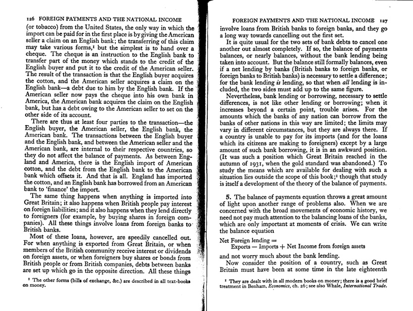
Here is a scan of two pages on the balance of payments – the topic I like the most.
(click to enlarge)
Hicks understood how weak balance of payments can cause troubles. Of course, it took the genius of Nicholas Kaldor to realize the supreme importance of balance of payments in the determination of national income and expenditure. Leaving that aside, the text has nice ideas and discussions on how stocks and flows feed into one another.
John Hicks is famous for an entirely different reason – the IS/LM model. Later he accepted it was a huge mistake, but put it mildly: “… as time as gone on, I have myself become dissatisfied with it”. But economists still keep using it and keep erring.
Also, Hicks was to soon abandon/forget his own social accounting approach as per Klamer-McCloskey’s article. Perhaps, not really.
In an extremely important paper, Wynne Godley said:
To come down to it, the present paper claims to have made, so far as I know for the first time, a rigorous synthesis of the theory of credit and money creation with that of income determination in the (Cambridge) Keynesian tradition. My belief is that nothing the paper contains would have been surprising or new to, say, Kaldor, Hicks, Joan Robinson or Kahn.
John Hicks also had another nice book called A Market Theory Of Money written in 1989. Here is a great insight (also the view of Kaldor) from Page 11, Chapter 1 named “Supply And Demand?” on how to create a dynamic Keynesian theory of determination of national income and expenditure:
… The traditional view that market price is, at least in some way, determined by an equation of demand and supply had now to be given up. If demand and supply are interpreted, as had formerly seemed to be sufficient, as flow demands and supplies coming from outsiders, it is no longer true that there is any tendency over any particular period, for them to be equalized: a difference between them, if it were not too large, could be matched by a change in stocks. It is of course true that if no distinction is made between demand from stockholders and demand from outside the market, demand and supply in that inclusive sense must be equal. But that equation is vacuous. It cannot be used to determine price, in Walras’ or Marshall’s manner. For what matters to the stockholder is the stock that he is holding: the increment in that stock, during a period is the difference between what is held at the end and what was held at the beginning, and the beginning stock is carried over from the past. So the demand-supply equation can only be used in a recursive manner, to determine a sequence (It is a difference or a differential equation); it cannot be used directly to determine price, as Walras and Marshall had used it.
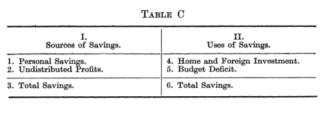
which is the now famous sectoral balances identity! Incidentally, it also includes Kalecki’s profit equation. In the above “Foreign Investment” shouldn’t be confused with Foreign Direct Investment flows in the financial account of the balance of payments. The authors define it as:
… equal to income generated by receipts from abroad less current expenditure abroad.
So can we call the profit equation SMK equation? 🙂
James Meade and Richard Stone were pioneers of national accounts. Incidentally, James Meade wrote a famous textbook on balance of payments.
Of course the way this is presented doesn’t make the connection between the financial account and current accounts. The sectoral balances was usually written by Wynne Godley as:
NAFA = PSBR + BP
where NAFA is the net accumulation of financial assets of the private sector, PSBR is the net public sector borrowing requirement, and BP is the current account balance of international payments. More on this connection below.
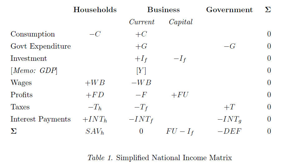
How it is to be derived in a stock-flow consistent framwork of Godley/Lavoie? If you click on this search Transactions Flow Matrix, you will find some blog posts on the background. First, we construct a flow matrix like this:
The last line is essentially Kalecki’s profit equation.
The above construction however raises an important question. Godley and Lavoie’s textbook (Chapter 2) quotes a famous 1949 article of Morris Copeland on this:
When total purchases of our national product increase, where does the money come from to finance them? When purchases of our national product decline, what becomes of the money that is not spent?
Copeland’s work was highly successful and established the flow of funds accounts of the United States in 1952.
Here is a republished version of the article (via Google Books):
click to preview on Google Books’ site
Incidentally, Copeland was motivated to prove the quantity theory of money wrong when he did this work! Also Godley/Lavoie point out that John Dawson (the editor of the above book) says:
the acceptance of…flow-of-funds accounting by academic economists has been an uphill battle because its implications run counter to a number of doctrines deeply embedded in the minds of economists.
in an article from the chapter The Conceptual Relation Of Flow-Of-Funds Accounts To The SNA of the same book.
Over time, the system of national accounts (with its first version in 1947) has used some of the concepts of flow of funds accounting and now the framework is much more wider than usual textbook guides of national accounts. The flow of funds still retains importance because it has information which the system of national accounts such as (2008 SNA) doesn’t handle.
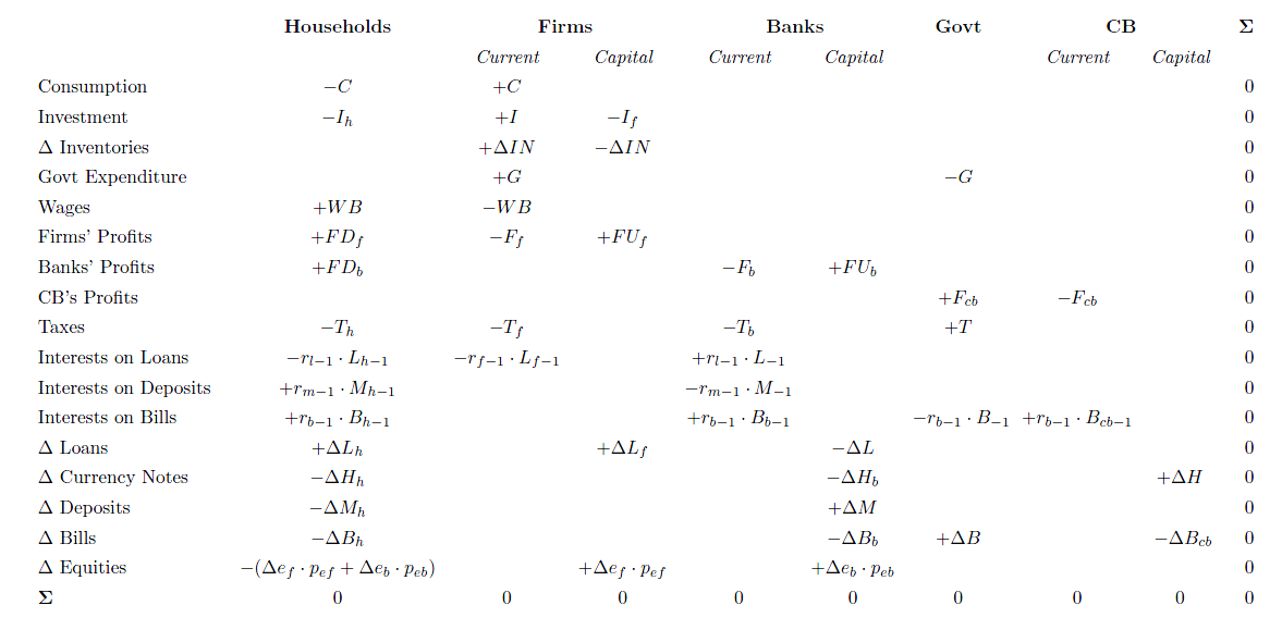
How does one look at this in a stock-flow coherent framework? Simple, we need a full transactions flow matrix – which not only includes income/expenditure flows but also financial flows. The following is how it looks like for a simple model:
Formally, prescribing a closure boils down to stating which variables are endogenous or exogenous in an equation system largely based upon macroeconomic accounting identities, and figuring out how they influence one another.
Of all the economists, Wynne Godley had the rarest of rare ability to model and imagine the economic dynamics of the whole world. “… a full macroeconomic model in his head, which, by some sort of subconscious process, he computed.” as his obituary from FT said.
In the recent INET conference paper, Dirk Bezemer discusses Wynne Godley’s approach (among others’) and also refers to his paper Seven Unsustainable Processes from 1999.
I obtained this original scanned copy of the paper Seven Unsustainable Processes – Medium Term Policies For The United States And The World by Wynne Godley from 1999 from the Levy Economics Institute and thought that since this version is missing for some reason from the levyinstitute.org website, I’ll post it here (after asking them if I may post).
Click to see the pdf.
Seven Unsustainable Processes from 1999
Here’s the link to the updated version of the paper from the year 2000. The original had a typo. Two columns in Table 1 appeared with incorrect headings (should have been the reverse).
Wynne Godley at the Levy Institute
Godley warns of the private sector indebtedness:
… Moreover, if, per impossibile, the growth in net lending and the growth in money supply growth were to continue for another eight years, the implied indebtedness of the private sector would then be so extremely large that a sensational day of reckoning could then be at hand.
Wynne Godley never liked the chimerical and primitive view of economists where anything and everything is traded in the markets via supply and demand. So,
The difference between the consensus view and that put forward here could not exist without a profound difference in the view of how the economy works. So far as the author can observe, the underlying theoretical perspective of the optimists, whether they realize it or not, sees all agents, including the government, as participants in a gigantic market process in which commodities, labor, and financial assets are supplied and demanded. If this market works properly, prices (e.g., for labor and commodities) get established that clear all markets, including the labor market, so that there can be no long-term unemployment and no depression. The only way in which unemployment can be reduced permanently, according to this view, is by making markets work better, say, by removing “rigidities” or improving flows of information. The government is a market participant like any other, its main distinguishing feature being that it can print money. Because the government cannot alter the market-clearing price of labor, there is no way in which fiscal or monetary policy can change aggregate employment and output, except temporarily (by creating false expectations) and perversely (because any interference will cause inflation).
No parody is intended. No other story would make sense of the assumption now commonly made that the balance between tax receipts and public spending has no permanent effect on the evolution of the aggregate demand. And nothing else would make sense of the debate now in full swing about how to “spend” the federal surplus as though this were a nest egg that can be preserved, spent, or squandered without any need to consider the macroeconomic consequences.
The seven unsustainable processes were:
(1) the fall in private saving into ever deeper negative territory, (2) the rise in the flow of net lending to the private sector, (3) the rise in the growth rate of the real money stock, (4) the rise in asset prices at a rate that far exceeds the growth of profits (or of GDP), (5) the rise in the budget surplus, (6) the rise in the current account deficit, (7) the increase in the United States’s net foreign indebtedness relative to GDP.
As it happened, the United States went into a recession but recovered quickly because of further deregulations and low interest rates which led to more borrowing, and a fiscal stimulus which put a floor on the downfall. However, the private sector went back into deficits and its indebtedness kept rising relative to income. The current balance of payments also went deeply in deficit rising to about 6.43% at the end of 2005 – hemorrhaging the circular flow of national income at a massive scale. See the related post here: The Un-Godley Private Sector Deficit.
Not only did Godley see the crisis coming, he also figured out that the United States will soon run into policy issues and will have less room to come out of a crisis. In this 2005 strategic analysis paper The United States And Her Creditors – Can The Symbiosis Last? he and his collaborators (Dimitri Papadimitriou, Claudio Dos Santos and Gennaro Zezza) pointed out that:
The range of strategic policy options for the United States is beginning to narrow … As the normal equilibrating forces (changes in exchange rates) are being subverted, it is very far from obvious what the United States can do on her own …
The prospects for the U.S. economy have become uniquely dreadful, if not frightening. In this paper we argue, as starkly as we can, that the United States and the rest of the world’s economies will not be able to achieve balanced growth and full employment unless they are able to agree upon and implement an entirely new way of running the global economy.
Stressing the need for concerted action (from which I got the title of my blog!), the authors said:
… Fiscal policy alone cannot, therefore, resolve the current crisis. A large enough stimulus will help counter the drop in private expenditure, reducing unemployment, but it will bring back a large and growing external imbalance, which will keep world growth on an unsustainable path …
… What must come to pass, perhaps obviously, is a worldwide recovery of output, combined with sustainable balances in international trade. Since this series of reports began in 1999, we have emphasized that, in the United States, sustained growth with full employment would eventually require both fiscal expansion and a rapid acceleration in net export demand. Part of the needed fiscal stimulus has already occurred, and much more (it seems) is immediately in prospect. But the U.S. balance of payments languishes, and a substantial and spontaneous recovery is now highly unlikely in view of the developing severe downturn in world trade and output … By our reckoning (which is put forward with great diffidence), if the United States were to attempt to restore full employment by fiscal and monetary means alone, the balance of payments deficit would rise over the next, say, three to four years, to 6 percent of GDP or more—that is, to a level that could not possibly be sustained for a long period, let alone indefinitely …
… It is inconceivable that such a large rebalancing could occur without a drastic change in the institutions responsible for running the world economy—a change that would involve placing far less than total reliance on market forces.
A commenter on my post on Net Worth asked me if I could do an example.
Here it goes.
First I do it as done by national accountants as per 2008 SNA – the System of National Accounts and then by the method used by the Federal Reserve’s Z.1 Flow of Funds Accounts.
The example is from a Levy Institute working paper by Antonio C. Macedo e Silva and Claudio Dos Santos with tables created more neatly here.
Let us assume that a single firm starts with the following balance sheet.
Opening Stocks: 2011
$
Assets
900
Nonfinancial Assets Financial Assets
600 300
Liabilities and Net Worth
900
Securities Other Than Shares Loans Shares and Other Equity Net Worth
150 250 450 50
In the above Net Worth is defined as we did earlier by treating equities as liabilities of a corporation. As we saw in the table Transactions Flow Matrix in the post Sources And Uses Of Funds, firms finance investment by retained earnings, and incurring liabilities. It was a simplified matrix of course and firms may also by sale of assets they hold.
An important point in the analysis is that this is for a single firm not the consolidated corporate sector as I am going to assume it will purchase physical capital from another firm for which it is a part of current receipts and hence a source of funds for the latter. That is, in the Transactions Flow Matrix, “I” appears both in the current and capital account of the consolidated production firms sector but here we are interested in a single firm.
Let us assume in an accounting period the firm retains $90 of earnings and finances a purchase of physical capital of $400 by this and issuing $50 net of corporate paper (net), taking $150 of new bank loans, issuing $40 of equities in the markets and selling existing financial assets worth $70.
The closing balance sheet will be as follows:
Closing Stocks: 2011
$
Assets
1,230
Nonfinancial Assets Financial Assets
1000 230
Liabilities and Net Worth
1,230
Securities Other Than Shares Loans Shares and Other Equity Net Worth
200 400 490 140
We assume away capital gains i.e., asset prices haven’t changed for the sake of clarity. As you see, net worth has increased from $50 to $140 and this is due to the firm’s saving – undistributed profits of $90. In general, asset prices change all the time and there will be holding gains and/or losses in both assets and liabilities.
What about flows such as the financial balance?
Here Saving = +$90
Net Incurrence of Liabilities = (+$50) + (+$150) + (+$40) = +$240
Net Acquisition (or Accumulation) of Financial Assets = (-$70)
because of the sale of assets and hence
Net Lending by the firm = (-$70) – (+$240) = (-$310)
(This is also called NAFA in old terminology, instead of splitting Net Lending into Net Accumulation of Financial Assets and Net Incurrence of Liabilities.)
To check: this is equal to Saving Minus Investment which is +$90 – $400 which is equal to -$310 – the “financial balance” of the firm.
So even though we have a negative financial balance, the firm’s net worth has increased. However note that by doing so, the firm’s financial assets/liabilities ratio has reduced – increasing its fragility somewhat.
As mentioned earlier, the purchase of physical capital was from another firm and we have not consolidated the corporate sector and hence the above balance sheets are for a single firm only.
Alternative Approach
The Federal Reserve will do this differently because equities issued by corporations are treated as if they are not liabilities in its Z.1 Flow of Funds Accounts of the United States and accordingly the example will need to be modified to look like this:
Opening Stocks: 2011
$
Assets
900
Nonfinancial Assets Financial Assets
600 300
Liabilities and Net Worth
900
Securities Other Than Shares Loans Net Worth Memo: Shares and Other Equity
150 250 500 450
I have added Equities in “Memo” as per the Federal Reserve’s practice and the Net Worth at the beginning of the period is $500. With the same set of transactions – a purchase of physical capital of $400 by this and issuing $50 net of corporate paper (net), taking $150 of new bank loans, issuing $40 of equities in the markets and selling existing financial assets worth $70, while retaining earnings of $90 in the period, the closing stocks will be as below:
Closing Stocks: 2011
$
Assets
1,230
Nonfinancial Assets Financial Assets
1000 230
Liabilities and Net Worth
1,230
Securities Other Than Shares Loans Net Worth Memo: Shares and Other Equity
200 400 630 490
Here Net Worth increased by $130 from $500 to $630 because of retained earnings of $90 and issuance of equities of $40 in the period.
The second approach is more like an “own funds” approach.
In the previous two posts, I went into a description of the transactions flow matrix and the balance sheet matrix as tools for an analytic study of a dynamical study of an economy.
During an accounting period, sectors in an economy are making all kinds of transactions. These can be divided into two kinds:
Income and Expenditure Flows
Financing Flows
Let’s have the transactions flow matrix as ready reference for the discussion below.
(Click for a nicer view in a new tab)
The matrix can easily be split into two – on top we have rows such as consumption, government expenditure and so on and in the bottom, we have items which have a “Δ” such as “Δ Loans” or “change in loans”. We shall call the former income and expenditure flows and the latter financing flows.
To get a better grip on the concept, let us describe household behaviour in an economy. Households receive wages (+WB) and dividends from production firms (called “firms” in the table) and banks (+FD_{f} and +FD_{b}) respectively) on their holdings of stock market equities. They also receive interest income from their bank deposits and government bills. These are sources of households’ income. While receiving income, they are paying taxes and consuming a part of their income (and wealth). They may also make other expenditure such as buying a house or a car. We call these income and expenditure flows.
Due to these decisions, they are either left with a surplus of funds or a deficit. Since we have clubbed all households into one sector, it is possible that some households are left with a surplus of funds and others are in deficit. Those who are in surplus, will allocate their funds into deposits, government bills and equities of production firms and banks. Those who are in deficit, will need funds and finance this by borrowing from the banking system. In addition, they may finance it by selling their existing holding of deposits, bills and equities. The rows with a “Δ” in the bottom part of transactions flow matrix capture these transactions. These flows will be called financing flows.
How do banks provide credit to households? Remember “loans make deposits”. See this thread Horizontalism for more on this.
This can be seen easily with the help of the transactions flow matrix!
The two tables are some modified version of tables from the book Monetary Economics by Wynne Godley and Marc Lavoie.
It is useful to define the flows NAFA, NIL and NL – Net Accumulation of Financial Assets, Net Incurrence of Liabilities and Net Lending, respectively.
If households’ income is higher than expenditure, they are net lenders to the rest of the world. The difference between income and expenditure is called Net Lending. If it is the other way around, they are net borrowers. We can use net borrowing or simply say that net lending is negative. Now, it’s possible and typically the case that if households are acquiring financial assets and incurring liabilities. So if their net lending is $10, it is possible they acquire financial assets worth $15 and borrow $5.
So the the identity relating the three flows is:
NL = NAFA – NIL
I have an example on this toward the end of this post.
I have kept the phrase “net” loosely defined, because it can be used in two senses. Also, some authors use NAFA when they actually mean NL – because previous system of accounts used this terminology as clarified by Claudio Dos Santos. I prefer old NAFA over NL, because it is suggestive of a dynamic, though the example at the end uses the 2008 SNA terminology.
While households acquire financial assets and incur liabilities, their balance sheets are changing. At the same time, they also see holding gains or losses in their portfolio of assets. What was still missing was a full integration matrix but that will be a topic for a post later. Since, it is important however, let me write a brief mnemonic:
where revaluations denotes holding gains or losses.
This is needed for all assets and liabilities and for all sectors and hence we need a full matrix.
We will discuss more on the behaviour of banks (and the financial system) and production firms some other time but let us briefly look at the government’s finances.
As we saw in the post Sources And Uses Of Funds, government’s expenditure is use of funds and the sources for funds is taxes, the central bank’s profits, and issue of bills (and bonds). Unlike households, however, the government is in a supreme position in the process of “money creation”. Except with notable exceptions such as in the Euro Area, the government has the power to make a draft at the central bank under extreme emergency, though ordinarily it is restricted. Wynne Godley and Francis Cripps described it as follows in their 1983 book Macroeconomics:
Our closed economy has a ‘central bank’ with two principle functions – to manage the government’s debt and to administer monetary policy. [Footnote: The central bank has to fund the government’s operations but this in itself presents no problems. Government cheques are universally accepted. When deposited with commercial banks the cheque become ‘reserve assets’ in the first instance; banks may immediately get rid of excess reserve assets by buying bonds.]. The only instrument of monetary policy available to the central bank in our simple system is the buying and selling of government bonds in the bond market. These operations are called open market operations. We assume that the central bank does not have the right to directly intervene directly in the affairs of commercial banks (e.g., to prescribe interest rates or quantitative lending limits) or to change the 10% minimum reserve requirement. But the central bank is in a very strong position in the bond market since it can sell or buy back bonds virtually without limit. This gives it the power, if it chooses, to fix bond prices and yields unilaterally at any level [Footnote: But speculation based on expectations of future yields may oblige the central bank to deal on a very large scale to achieve this objective.] and thereby (as we shall soon see) determine the general level of interest rates in the commercial banking system.
Given such powers, we can assume in many descriptions that the government’s expenditure and the tax rate is exogenous. However, many times, there are many constraints such as price and wage rises, high capacity utilization and low production capacity and also constraints brought about from the external sector due to which fiscal policy has to give in and become endogenous.
While I haven’t introduced open economy macroeconomics in this blog in a stock-flow coherent framework, we can make some general observations:
For a closed economy as a whole, income = expenditure. While it is true for the whole economy (worth stressing again: closed), it is not true for individual sectors. The household sector, for example, typically has its income higher than expenditure. In the last 15-20 years, even this has not been the case. If one sector has it’s income higher than expenditure, some sectors in the rest of the world will have its income lower than its expenditure. Many times, the government has its income lower than expenditure and we see misleading public debates on why the government should aim to achieve a balanced budget. When a sector has its income lesser than expenditure, it’s net lending is negative and hence is a net borrower from the rest of the world. It can finance this by borrowing or sale of assets. A region or a whole nation can have its expenditure higher than income and this is financed by borrowing from the rest of the world. A negative flow of net lending implies a net incurrence of liabilities – thus adding to the stock of net indebtedness which can run into an unsustainable territory. Stock-flow coherent Keynesian models have the power to go beyond short-run Keynesian analysis and study sustainable and unsustainable processes.
… it is important to have in mind that it is possible to get three kinds of trajectories with SFC models:
trajectories toward a sustainable steady state;
trajectories toward a steady state over certain limits;
explosive trajectories.
The analysis of SFC models’ dynamic trajectories and steady states is useful, first because it makes clear to the analyst whether the regime described in the model is sustainable or whether it leads to some kind of rupture—either because the trajectory is explosive or because it leads to politically unacceptable configurations. In these cases, as Keynes would say in the Tract, the analyst can conclude that something will have to change and even get clues about (i) what will probably change (since the sensitivity of the system dynamics to changes in different behavioural parameters is not the same); and (ii) when this change will occur (since the system may converge or diverge more or less rapidly).
Example
Note that Net Lending is different from “saving”. Say, a household earns $100 in a year (including interest payments and dividends), pays taxes of $20 and consumes $75 and takes a loan of to finance a house purchase near the end of the year whose price is $500. Assume that the Loan-To-Value (LTV) of the loan is 90% – which means he gets a loan of $450 and has to pay the remaining $50 from his pocket to buy the house. (i.e., he is financing the house mainly by borrowing and partly by sale of assets). How does the bank lending – simply by expanding it’s balance sheet (“loans make deposits”). Ignoring, interest and principal payments (which we assume to fall in the next accounting period),
His saving is +$100 – $20 – $75 = +$5.
His Investment is +$500.
His Net Incurrence of Liabilities is +$450.
His Net Accumulation of Financial Assets is +$5 – $50 = – $45.
His Net Lending is = -$45 – (+$450) = -$495 which is Saving net of Investment ($5 minus $500).
This means even though the person has “saved” $5, he has incurred an additional liability of $450 and due to sale of assets worth $45, he is a net borrower of $495 from other sectors (i.e., his net lending is -$495).
Assume he started with a net worth of $200.
Opening Stocks: 2010
$
Assets
200
Nonfinancial Assets Deposits Equities
0 30 170
Liabilities and Net Worth
200
Loans Net Worth
0 200
Now as per our description above, the person has a saving of $5 and he purchases a house worth $500 by taking a loan of $450 and selling assets worth $50. We saw that the person’s Net Accumulation of financial assets is minus $45. How does he allocate this? (Or unallocate $45)? We assume a withdrawal of $10 of deposits and equities worth $35. At the same time, during the period, assume he had a holding gain of $20 in his equities due to a rise in stock markets.
Hence his deposits reduce by $10 from $30 to $20. His holding of equities decreases by $15 (-$35 + $20 = -$15)
How does his end of period balance sheet look like? (We assume as mentioned before that the purchase of the house occurred near the end of the accounting period, so that principal and interest payments complications appear in the next quarter.)
Closing Stocks: 2010
$
Assets
675
Nonfinancial Assets Deposits Equities
500 20 155
Liabilities and Net Worth
675
Loans Net Worth
450 225
Just to check: Saving and capital gains added $5 and $20 to his net worth and hence his net worth increased to $225 from $200.
Of course, from the analysis which was mainly to establish the connections between stocks and flows seems insufficient to address what can go wrong if anything can go wrong. In the above example, the household’s net worth gained even though he was incurring a huge liability. What role does fiscal policy have? The above is not sufficient to answer this. Hence a more behavioural analysis for the whole economy is needed which is what stock-flow consistent modeling is about.
One immediate answer that may satisfy the reader now is that the households’ financial assets versus liabilities has somewhat deteriorated and hence increased his financial fragility. By running a deficit of $495 i.e., 495% of his income, the person and his lender has contributed to risk. Of course, this is just one time for the person – he may be highly creditworthy and his deficit spending is an injection of demand which is good for the whole economy. After all, economies run on credit. While this person is a huge deficit spender, there are other households who are in surplus and this can cancel out. In the last 15 years or so, however (before the financial crisis hit), households (as a sector) in many advanced economies ran deficits of the order of a few percentage of GDP. If the whole household sector continues to be a net borrower for many periods, then this process can turn unsustainable as the financial crisis in the US proved.
Now to the title of the post. Flows such as consumption, taxes, investment are income/expenditure flows. Flows such as “Δ Loans”, “Δ Deposits”, “Δ Equities” are financing flows. Income/expenditure flows affect financing flows which then affect balance sheets, as we see in the example.
 Happy reading!