In one of my recent posts, Saving Net Of Investment, I went into gross saving versus saving net of consumption of fixed capital. I showed how depreciation – or more appropriately, consumption of fixed capital – is treated in the flow of funds accounts.
Since the transactions flow matrix is a powerful tool for visualizing flow of funds, the question is where depreciation makes an appearance. The following table created by me using shows how for a simple economy.
FIGURE 1. Transactions Flow Matrix (click to enlarge)
Here “Firms” is a shorthand for all production firms as a sector and I took the consumption of fixed capital of firms only for illustration purposes. (Else I would have needed to break the households’ accounts into current and capital accounts – eating up space).
Investment here is gross investment and consumption of fixed capital makes its appearance in the line 3. It is a negative item in the current account and a positive item in the capital account. So it more of a book-keeping device but an important one because depreciation is not unimportant. The definition of profits is that of Wynne Godley and is slightly different from National Accounts. Also, while undistributed profits is a source of funds, CFC is also!
So undistributed profits (FU) and consumption of fixed capital (CFC) are both sources of funds. (Positive signs denote sources of funds and negative – uses of funds). This can be confusing because depreciation is a negative for net worth. The reason is that, as I have mentioned before, revaluations need to be done before end of period stocks are calculated. And it is where consumption of fixed capital will make a reappearance – subtracting from net worth due to a reduction in the value of nonfinancial assets.
It is important to keep in mind that equities are also sources of funds as the last line (above Σ) shows. So net saving (undistributed profits for firms) and consumption of fixed capital add to changes in net worth. (Note: Net is net of consumption of fixed capital here and not net of investment!).
This can be seen from the UK Blue Book 2011.
FIGURE 2. UK Blue Book 2011 Accumulation Accounts (click to enlarge)
A Digression
What is the origin of the confusing phrase “net saving” – saving net of investment? I believe it came from Nicholas Kaldor himself who originated the sectoral balances approach. Here’s from The Scourge Of Monetarism, 1982, pp 48-50:
The PSBR in any year can be defined as the public sector’s net de-cumulation of financial assets (net dissaving) which by accounting identity must be equal to the net acquisition of financial assets (net saving) of the private sector, home and overseas; which in turn can be broken down to the net acquisition of financial assets of the personal sector, of the company sector, and the overseas sector (the latter is the negative of the balance of payments on current account).
In a recent paper, Bradford DeLong and Lawrence Summers suggest that a fiscal expansion can be useful to bring an economy from a depressed state (!). The rough idea being that a relaxation of fiscal policy leads to a higher output and the increase in economic activity leads to a stabilization of public debt/gdp ratio.
This condition is valid as long as (in the authors’ terminology):
(click to enlarge)
The interesting thing about this is that the authors suggest that even if r > g, it is possible for the public debt/gdp to remain sustainable under certain conditions.
I won’t have more to say on this because it uses a standard one-period analysis but the fact that some mainstream authors seem to understand the fiscal policy dynamics better is encouraging.
Arguing that their “… conclusions conflict with those of the “new consensus,” which holds that a correct setting of interest rates is the necessary and sufficient condition for achieving noninflationary growth at full employment, leaving fiscal policy rather in the air.”, they also derive a result for a closed economy:
It is usually asserted that, for the debt dynamics to remain sustainable, the real rate of interest must be lower than the real rate of growth of the economy for a given ratio of primary budget surplus to gdp. If this condition is not fulfilled, the government needs to pursue a discretionary policy that aims to achieve a sufficiently large primary surplus. We can easily demonstrate that there are no such requirements in a fully consistent stock-flow model such as ours.
The G&L style of modeling is extremely useful because it gives great attention to stocks and flows so that no errors creep in. The result is surprising the first time one hears this because it goes against intuition. This can be seen by thinking of the interest payments of the government as income for the domestic private sector!
So no conditions such as r < g!
Open Economy Debt Dynamics
For open economies, G&L are also able to construct select scenarios where a debtor nation can be indebted to the rest of the world without the nation’s debt (which is different from public debt) increasing relative to gdp forever. (Of course by no means proving/implying it for all possible scenarios).
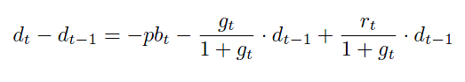
where d is “external debt” and pb is the primary balance of the current account balance. (The expressions are relative to gdp)
Suppose the government and the central bank want to restrict external debt to 50% of gdp – with the view that foreigners may consider moving above it as unsustainable. Assume growth is 3.5% and effective interest rate paid on liabilities to foreigners is 1%. Then the tolerable primary deficit of current account balance is 1.25%. This is calculated by setting the left hand side to zero and just plugging the formulas. (See below)
Please note, a higher growth will worsen the external balance so it is not a good argument that growth can lead to a lower debt/gdp ratio.
To summarize, intuitions for a closed economy and the open economy can appear contradictory.
Standard Analysis
I have seen many economists including Post Keynesians (not G&L) take the above equation and interpret it rather differently. So assuming sustainability, a constant primary balance pb implies the debt sustains at
or simply,
A continuous time formulation leads to an equality sign. The above is derived by assuming the debt sustains at d and shuffling the terms in the first equation.
Note: the above is valid only if there a stabilization. Else, in the case where g < r, the above expression gives a negative answer for a negative primary balance – but that is because the derivation assumed sustainability and cannot be used when debt/gdp keeps rising.
This is also written sometimes as
by expanding the denominator of the previous expression using the Taylor Theorem from Mathematics.
This raises a curiosity – how come in the G&L case for the closed economy did the debt sustain even when g > r? That’s because it was a dynamic stock-flow consistent model as opposed to the artificial assumption of a constant deficit used in standard analysis such as the third equation above.
Nonetheless the above analysis shows that for a constant deficit (though artificial), debt sustains as per the equation (assuming growth and the rate of interest paid are constant as well!)
Back to Open Economies
Moving to the open economy case, where debt and deficit denote the external debt and the current account deficit, the above shows that if the primary deficit is restricted somehow to say 5% of gdp and the differential between growth and interest rate is 2%, the external debt sustains at 250% of gdp.
This should be seen as a restriction. Instead some/many Post Keynesians just state it is sustainable. A higher growth rate will increase the deficit (current account) and the debt-dynamics can make the whole process unsustainable. So one needs to model how fiscal policy itself affects the current account deficit rather than keeping it a constant relative to gdp.
This is the reason many nations find themselves troubled by the external sector.
This can be seen for the case of the United States. A huge relaxation of fiscal policy will bring back the current account deficit to 6% of gdp (and rising) and put the world on an unsustainable path. What the United States needs to do is ask its trading partners to expand domestic demand by fiscal expansion and achieve higher growth so that it itself can achieve a higher growth rate due to the extra space created for fiscal policy.
More generally, we need a concerted action!
For a related analysis see Dean Baker’s recent analysis on the trade deficit being America’s fundamental imbalance: The Iron Grip of Accounting Identities
Summary
There is no condition such as if r <g, debt is sustainable. Debt can keep rising relative to gdp simply because deficit keeps rising.
The condition r > g can be useful in studying certain circumstances for analysis.
Money is endogenous and is created as a byproduct of the production process. I came across this reference which supposedly shows that there is supposedly a one-to-one relationship between money and inflation and hence as a consequence – if we were to believe this – if the Bureau of Engraving and Printing were to work extra-time, this would lead to high inflation!
This is a highly misleading. Borrowing to produce something leads to an increase in demand and wealth and the private sector allocates its financial wealth into deposits and various securities. So money is a residual. Some of the increase in demand spills over to price rise and in exceptional cases can run out of control because of other reasons as well, leading to more borrowing and hence a growth in the money stock and higher inflation. But it is misleading to say that the growth of the money stock caused the inflation.
The reference is Some Monetary Facts from the Summer 1995 Quarterly review of the Federal Reserve Bank of Minneapolis which makes confusing statements about what the central bank does or should do. Here’s a graph from the paper supposedly establishing a connection between growth in the money stock and inflation. I added the pink line to make it look less scary 🙂
The points in the graph are average growth rates of the money stock and price rises for 110 countries.
According to the authors, the correlation is around 0.95 and the 45° line supposedly shows the tight link between money and inflation.
God we are in for a very high inflation soon!
This correlation analysis can easily be produced by creating a data set with the same properties (high correlation, 45 degree line etc) and I was able to do so below:
The slope is nearly 1 (0.97) and a correlation of 0.97 (even better!).
When you look at the individual data, you will see that except countries with very high inflation, there is hardly any issue.
If you were to remove the points with high inflation, the “monetary facts” as per the authors go away.
Of course, did money (or central bank open market operations) cause inflation in those countries – of course not. Money is a residual.
How does the M2/CPI look for the United States? Here’s the monthly graph of the ratio, with M2 in billions of dollars and CPI defined so that is equal to 100 in 2005. This following shows how wrong the “Monetarist intuition” is. Money didn’t increase one-to-one with prices and the ratio has grown from 35.8 to 82.7.
(Data Source: Federal Reserve Bank of St. Louis)
Note: The data in the excel sheet was created using random data and some amount of tweaks by me to reach the graph similar to the original Minneapolis Fed paper. So it is an imaginary data set created to have similar properties.
At the risk of boring readers, here’s Bundesbank’s TARGET2 claims again from its March 2012 Monthly Report. Cannot find the English version but the translation is below the first figure (with old data). This increased to almost €560bn at the end of February despite ease in financial market conditions in the Euro Area!
(click to enlarge)
English translation from an older report:
(click to enlarge)
As mentioned earlier these arise due to capital flight into Germany from the “periphery” countries.
Some economists and financial analysts try to downplay this by saying that in reality the actual loss (in case of a breakup of the Euro Area and subsequent default by the periphery) to Bundesbank and hence Germany is lesser and this number should be multiplied by the capital key. For Bundesbank this is 18.9373% and using the February number this amounts to a maximum loss of €106bn as per this calculation.
This is misleading to the core. Firstly if the debtor nations default the creditor nations suffer in full. So if Bundesbank’s losses are low, other creditor nations’ losses will be high. Also, Bundesbank suffers due to losses incurred by other NCBs of creditor nations such as Belgium since these losses are shared. Secondly, the capital key would be some sort of weighted key among the creditor nations’ central banks and will be higher.
At any rate, the creditor nation lose the full amount of the claim of the ECB on the periphery nations in the case of a breakup. This number can vastly increase if there is a panic and further capital flight into the “core”. Of course, there will be other losses and costs of a breakup but IMO – nonetheless this is not unimportant.
Having said this, these things are very unpredictable – it is perfectly possible that a boom in financial markets for whatever reasons reverses the flight making the unsustainable process run longer than one may think. It is also possible – as Euro Area leaders have been planning wittingly or unwittingly – that trade is balanced internally by deflating demand in debtor nations and but this will come with a lower output and higher unemployment in general and injures all alike.
The above increase could also have been because banks in nations such as Spain may have redeemed some of their liabilities to banks in Germany and refinanced themselves via the three-year LTRO in February.
The commenter JKH has an outstanding post here at Cullen Roche’s blog criticizing the Neochartalists’ mixing up of saving and saving net of investment.
JKH quoting Randy Wray:
Then, this is telling:
“To briefly summarize, at NEP we prefer to use the Godley sectoral balance approach, where he defined private sector saving as “net accumulation of financial assets” (NAFA), using the flow of funds data. Typically economists use the GDP equals national income equation where saving is defined as a residual: the net income received but not consumed (I’ll use it below in discussing the MMR approach). In theory these would lead to approximately the same result; in practice they do not because the NIPA accounts include imputed values. Godley preferred the flow of funds data but even they had to be carefully adjusted to ensure that every spending flow is actually financed and actually “goes somewhere” (ensuring “stock-flow consistency”). That is all quite wonky. My bigger point is that we can come up with alternative definitions of saving that would include unrealized capital gains as real and financial assets appreciate in value.”
This seals the case regarding MMT’s confused interpretation of the term “saving”. I don’t know if that correctly reflects what Godley does or not, but if private sector saving is defined that way it has nothing to do with the private sector saving S that’s cast in MMT’s own 3 sector financial balances model. S cannot identically equal (S – I) unless I is identically zero, which is ridiculous.
For example, in a closed economy with a balanced budget, if the (alleged) Godley definition of private sector saving is combined with the explicit definition of private sector saving S in the 3 sector SFB equation, then saving must be identically zero, whatever the level of investment. In cannot be otherwise for the Godley and MMT SFB specifications of S to be consistent. And in the real world economy, any such consistency would force global S = 0. And this is the point of it all – such inconsistency in the use of the term “saving” is fundamentally misleading.
Remarkably, Wray just demonstrated the same conflation of saving and net saving in MMT language and logic that is at the heart of the issue in question, which I find flabbergasting in the circumstances. Furthermore, he suggests this is consistent with the NIPA definition of saving. The definition of saving (allegedly) attributed to Godley above is not the same as NIPA defined saving at all. And the issue of imputed values or capital gains has nothing to do with the primary question. That is a secondary consideration having to do with the reconciliation of stocks and flows, not the outright confusion of flow definitions. It is a trees rather than a forest issue.
Of course this is an erroneous application of Godley’s sectoral financial balances approach as JKH himself suspects.
Wynne Godley never
… defined private sector saving as “net accumulation of financial assets” (NAFA), using the flow of funds data
and always specified that it is Net Saving which is NAFA and always specified Net Saving is Saving Net of Investment.
Excellent post by JKH exactly pinpointing to mixing terminologies and taking great pains to explain saving as an income residual.
JKH on me
Special mention also goes to Ramanan, who is a persistent seeker of accuracy when it comes to the subject more generally.
I had a post a month ago Banco de España’s TARGET2 Liabilities and this gets more interesting a month later. The bank released numbers for February and it seems capital flight is continuing from Spain and Spanish banks’ borrowing from the ECB rose in February. The following is from BdE
(click to enlarge)
The Spanish general government debt also continues to rise
(click to enlarge)
With Spain’s net indebtedness (not gross government debt) of €995bn to the rest of the world and having surrendered monetary sovereignty, this is not the best time for the nation – to say the least!
My last post was on U.S. net income payments from abroad and how it continues to be in the favour of the United States. The late Wynne Godley had been analyzing this since 1994. In an article titled U.S. Trade Deficits: The Recovery’s Dark Side?, written with William Milberg, he had a section called “Foreign indebtedness and the foreign income paradox” where he said:
So far, the practical consequences of the United States having become “the world’s largest debtor” have not been all that significant… But it would be an error to suppose that, because the net return on net assets has been negligible in the recent past, the same thing will be true in the future…
… Why did the net foreign income flow remain positive for so long after 1988? In order to understand this apparent paradox, it is essential to disaggregate stocks of assets and liabilities and their associated flows, and to distinguish (in particular) between financial assets and direct investments… The reason that net foreign income remained positive for so long can now be understood (at least up to a point) by making a comparison of the flows shown in Figure 3 with the stocks shown in Figure 2. The net inflow that arises from direct investment has been roughly equal to the net outflow on financial assets in recent years, even though the stock of financial liabilities has been about five times as large as the market value of net foreign investments. In other words, the rate of return on net direct investments far exceeded the rate on net financial liabilities
Figure 2 referred to is below:
and Figure 3:
which is what I redrew with updated data in my previous post. But as we saw the net income payments from abroad continues to be positive (!!) even till date but the reason is similar. Foreign direct investment in the United States has risen to $2.8T at the end of 2011 as per Federal Reserve’s Z.1 Flow of Funds while U.S direct investment abroad rose to $4.8T – significantly higher (even as a percent of GDP) than in the mid-90s.
The net direct investment has seen huge returns (both via income and holding gains) and so this killing has brought in good fortunes for the United States. Of course with the whole current account of balance of payments in deficit, the external sector bleeds the circular flow of national income in the United States and contributes to weak demand there.
So a current account deficit is bad for the United States but financing this deficit has been easy for the United States given that the US Dollar is the reserve currency of the world. Why do nations require reserve assets? The late Joseph Gold of the IMF gave a nice description in his book Legal and Institutional Aspects of the International Monetary System: Selected Essays:
click to view on Google Books
What makes the US dollar the reserve currency of the world is difficult to argue. However it cannot be taken for granted that the United States may enjoy this exorbitant privilege given that the Sterling was once the darling of the financial markets and central banks.
Their argument is similar – direct investments have made huge returns for the domestic private sector of the United States and gives a good account of the external sector. Here’s a graph of the United States’ net international investment position using data reported by the Federal Reserve’s Z.1 Flow of Funds Accounts as well as the BEA’s International Investment Position:
Why the difference is a topic for another post. I don’t know it yet. Gourinchas and Rey have some answers. The Federal Reserve’s data is till 2011 end and quarterly (and seasonally adjusted) while BEA data is yearly and available till 2010.
So, from the graph above, the United States became a net debtor of the world around 1986. The indebtedness has been rising mainly due to the huge current account deficits the nation manages to run and is partly offset by “holding gains”.
Here’s a graph of the current account deficit plotted with other “financial balances” (since they are related by an identity)
By the way, the U.S. was a creditor of the world when the Bretton Woods system of fixed exchange rates collapsed. Some authors describe this collapse by saying that money has become fiat since 1971 – whatever that means!
Gourinchas and Rey point out – correctly in my opinion:
The previous discussion points to a possible instability, even in an international monetary system that lacks a formal anchor. The relevant reference here is Triffin’s prescient work on the fundamental instability of the Bretton Woods system (see Triffin 1960). Triffin saw that in a world where the fluctuations in gold supply were dictated by the vagaries of discoveries in South Africa or the destabilizing schemes of Soviet Russia, but in any case unable to grow with world demand for liquidity, the demand for the dollar was bound to eventually exceed the gold reserves of the Federal Reserve. This left the door open for a run on the dollar. Interestingly, the current situation can be seen in a similar light: in a world where the United States can supply the international currency at will and invests it in illiquid assets, it still faces a confidence risk. There could be a run on the dollar not because investors would fear an abandonment of the gold parity, as in the 1970s, but because they would fear a plunge in the dollar exchange rate. In other words, Triffin’s analysis does not have to rely on the gold-dollar parity to be relevant. Gold or not, the specter of the Triffin dilemma may still be haunting us!
Gourinchas and Rey’s arguments depend on estimating a tipping point – the point where the net income payments from abroad turn negative. This of course depends on various assumptions but let us look at it.
The gross assets of the United States held abroad and liabilities to foreigners keep changing as the nation is able to increase its liabilities and use it to make direct investments abroad. The reserve currency status has provided the nation with this privilege as central banks around the world are willing to hold dollar-denominated assets. The positive return (as well as revaluation gains from the depreciation of the dollar – when it depreciates) helps reduce the net indebtedness but the current account deficit contributes to increasing it.
The following is the graph of gross assets and liabilities – using the Federal Reserve’s Z.1 Flow of Funds Accounts data and also BEA’s data for the ratio:
So assuming assets held abroad A make a return rA and liabilities L to foreigners lead to payments at an effective interest rate rL income payments from abroad will turn negative whenever
rA · A − rL · L < 0
So A and L are changing due to the current account deficits and revaluation gains on assets and liabilities. Meanwhile, the effective interest rates are themselves changing in time because of various things such as short term interest rates set by the central banks, market conditions, state of the economy etc. Also, if the private sector of the United States makes more direct investments abroad, this will contribute to increase rA (if successful) and the process can go on with net income payments from abroad staying positive for longer. The tipping point is defined by Gourinchas and Rey as the ratio L/A beyond which the the net income payments turn negative. According to their analysis (based purely on historical data), this is 1.30.
If the net income payments from abroad turns negative, international financial markets and central banks may start suspecting the future of the exorbitant privilege according to the authors. Of course, it may be the case that even if it turns negative, the United States’ creditors don’t mind – this has been the case of Australia. The following is from the page 18 of the Australian Bureau of Statistics release Balance of Payments and International Investment Position, Australia, Dec 2011 and in their terminology – which is the same as the IMF’s – it is called “net primary income”)
(Australia’s Q4 2011 GDP was around A$369bn for comparison) and the above graph is quarterly.
So, to conclude the process can continue as long as foreigners do not mind. It shouldn’t be forgotten however that Australian banks had funding issues during the financial crisis and the RBA used its line of credit at the Federal Reserve via fx swaps to prevent a run on Australian banks and it is difficult to design policy without keeping in mind the possibility of walking into uncharted territory.
Once net primary income turns negative, the process can quickly run into unsustainable territory due to the magic of compounding of interest unless the currency depreciates in the favour of the nation helping exports. Else demand has to be curtailed to prevent an explosion but this hurts employment. Other policy options include promotion of exports and asking trading partners to increase domestic demand by fiscal expansion.
The world economy has grown over the last so many years with the United States acting as the importer of the last resort. However, the U.S. current account deficit acts to bleed the circular flow of national income and weakens demand in the States. The nation still grew because of a huge lending boom.
Today, the U.S. Bureau of Economic Analysis came out with the Q4 report on the U.S. International Transactions. According to the release,
The U.S. current-account deficit—the combined balances on trade in goods and services, income, and net unilateral current transfers—increased to $124.1 billion (preliminary) in the fourth quarter of 2011, from $107.6 billion (revised) in the third quarter. Most of the increase in the current account deficit was due to a decrease in the surplus on income and an increase in the deficit on goods and services.
So the current account balance also consists of “income payments from abroad” – a bit of wrong phrasing because all items are income/expenditure flows. The net income payments from abroad continues to surprise analysts because in spite of the net indebtedness position of the United States, this continues to be positive and in recent times has increased! (although it fell the last quarter). Many hold the belief that the United States has lower interest rates and this is the consequence of that. While it is true that interest rates outside the U.S. are in general higher, and there is some truth to the above argument, it gives one the wrong impression that it will always be the case that net income from abroad will always be positive.
The following graph shows that this intuition is misleading. Most of the contribution to the net income is due to direct investments abroad which has made a killing for the private sector and the reverse – direct investment receipts for foreigners has made next to nothing. The remaining – income from financial assets held abroad less interest/dividend paid to foreigners’ holding of U.S. financial assets is already negative!
The red line has reduced in recent times due to lower interest rates in the U.S. presumably. But the more the U.S. continues to run large current account deficits, the deeper the red line will grow – pulling the black line to zero and into the negative territory.
The net income payments from abroad is more a result of the huge killing the U.S. domestic private sector has made abroad than because of lower interest rates. For example, excluding FDI, the data from BEA suggests that the “effective interest rate” on U.S. liabilities was 1.42% in 2010, while that on U.S assets held abroad is 1.65%. This differential will not be sufficient to keep the income payments to foreigners bounded. I used the 2010 data because the International Investment Position is available only till 2010 and the one for end of 2011 will be released only mid-2012.
To understand this, consider the case when the U.S net indebtedness grows to something about 100% of GDP due to the continuous current account deficits – if market forces allow the whole process to go on(!). This is an involved analysis involving some growth assumptions and the fiscal stance in the U.S. and the rest of the world. For example, people frequently forget that a higher growth in the U.S. will also bring in higher current account deficits. But it can easily be shown that the red and the black lines above grow into a negative territory if the United States wants to quickly achieve full employment by fiscal policy alone.
Of course the above graph shows that there is a lot fiscal expansion can achieve in the medium term for the United States.
These numbers look “small” and can lead one into believing that “all is well”. And this is another mistaken view. For example if there is a drastic relaxation of fiscal policy by the U.S. government, the current account deficit will soon hit 6-8% of GDP which may require further relaxation of fiscal expansion to compensate the leakage of demand due to the current account deficit and with income payments turning negative due to higher indebtedness, this will turn into an unsustainable path because the current account deficits and net indebtedness will keep increasing relative to GDP. This will need interest rate hikes to attract foreigners but turns the whole process unsustainable unless one believes in the foreign exchange market doing the trick. Also currently the interest rates are low because the Federal Reserve has kept them artificially low and foreigners do not mind holding U.S. dollar assets at this rate. As William Dudley says interest rates will be raised at some point by the Federal Reserve and this will increase payments to foreigners. See this post William Dudley On U.S. Sectoral Balances
Of course, this is not the only scenario and there’s a lot fiscal policy can achieve in the medium term but it is important to keep in mind that something needs to be done with the external sector to bring the external sector in balance to achieve full employment.
In my post The Transactions Flow Matrix, I went into how a full transactions flow matrix can be constructed using a simplified national income matrix. Let us reanalyze the latter. The following is the same matrix with some modifications – firms retain earnings and there are interest payments.
FU is the undistributed profits of firms. From the last line we immediately see that
SAVh + FU – If – DEF = 0
or that
FU = If + DEF – SAVh
This is Kalecki’s profit equation which says among other things that firms’ retained earnings is related to the government deficit! The equation appears in pages 82-83 of the following book by Michal Kalecki:
click to view on Google Books
In their book Monetary Economics, Wynne Godley and Marc Lavoie say this in a footnote:
Note that neo-classical economists don’t even get close to this equation, for otherwise, through equation (2.4), they would have been able to rediscover Kalecki’s (1971: 82–3) famous equation which says that profits are the sum of capitalist investment, capitalist consumption expenditures and government deficit, minus workers’ saving. Rewriting equation (2.3), we obtain:
FU = If + DEF − SAVh
which says that the retained earnings of firms are equal to the investment of firms plus the government deficit minus household saving. Thus, in contrast to neo-liberal thinking, the above equation implies that the larger the government deficit, the larger the retained earnings of firms; also the larger the saving of households, the smaller the retained earnings of firms, provided the left-out terms are kept constant. Of course the given equation also features the well-known relationship between investment and profits, whereby actual investment expenditures determine the realized level of retained earnings.
The above can of course also be written as:
I = SAVh + SAVf + SAVg = SAV
if one realized that the retained earning of firms is also their saving:
SAVf = FU
Business accountants know the connection between retained earnings and shareholders’ equity and in our language – which is that of national accountants/2008 SNA – it adds to their net worth just like household saving adds to their net worth.
Assuming away capital gains, we know from many posts that:
Change in Net Worth = Saving
Where do we find the undistributed profits in the Federal Reserve’s Flow of Funds Statistic Z.1?
In Table F.102, there’s an item called “Total Internal Funds”:
This is the first part of a series of posts I intend to write on the “rest of the world” accounts in National Accounts. This blog is about looking at economies from the point of view of National Accounts, Cambridge Keynesianism and Horizontalism. While various descriptions of balance of payments exist, most of them simply end up making money exogeneity assumption somewhere in the description!
In my view a careful description of balance of payments offers great insights on how economies work and what money really is. It is impossible to understand the success and failures of nations without understanding the external sector.
A description in terms of stocks and flows is the most appropriate for macroeconomics. Fortunately, national accountants have a good systematic approach to this.
Consider the following transaction: a government (or a corporation) raises funds in the international markets. The buyers can be residents as well as non-residents. The currency of the new issuance can be domestic as well as foreign. Does this by itself increase the net indebtedness of the nation as a whole?
The answer is No, and can be a bit surprising to the reader because the answer is the same whether the currency is domestic or foreign. The trick in the question is that an issuance of debt increases the assets and liabilities of the issuer!
(Note: the question was about the transaction, not on what happens after this)
Gross assets and liabilities vis-à-vis the rest of the world can be a bit more complicated and we need a more systematic analysis.
Consider another transaction. A government is redeeming a 7% bond with a notional of 1bn with semi-annual coupons. How much does the net indebtedness of the country change? Assuming that all the lenders are in the rest of the world sector, the net indebtedness changes by 35m. Does not matter if the currency is domestic or not. Why 35m? Because the semi-annual coupon has to be paid on redemption and the coupons are interest payments and this is recorded in the current account and this increases the net indebtedness. The principal payment cancels out the earlier liability – the bonds.
So between the start and the end of the period, foreigners earned 35m and this increased the net indebtedness of the nation who paid the interest. Of course there are other transactions which can cancel this out.
In another scenario, if all the bond holders were residents, the net indebtedness does not change – whether the bonds were in domestic currency or not.
The above was about financing. What about imports and exports? Exports provide income to a nation or a region as a whole and imports are opposite. If a nation is a net importer (more appropriately running a current account deficit), this means its expenditure is higher than income. When expenditure is higher than income, this has to be financed and this is via net borrowing.
There is one important point worth stressing. Many people – including many economists (most?) – treat liabilities to foreigners in domestic currency as not really a liability at all – at least the government’s liabilities. The reason provided is that while usually the government is forbidden from making an overdraft at the central bank or have limited powers in using central bank credit, it can end up making a higher use of it than the limits allowed – in extreme conditions. This in my opinion, is a silly intuition.
While it is true that the governments of most nations (with exceptions such as the Euro Area governments) can make a draft at the central bank and this offers the government protection to tide over extreme emergencies, the government has to directly or indirectly finance the current account deficits and this can prove unsustainable. Despite this there is an advantage in having indebtedness to foreigners in the domestic currency because:
An indebtedness to foreigners in domestic currency prevents revaluation losses on the debt if foreigners continue holding the debt and if the currency depreciates against foreign currencies. If the debt is denominated in a foreign currency and if it depreciates, more income needs to be earned from abroad to service the principal and interest payments.
The discussion can be confusing because of the relative ease with which the United States has managed till now to finance its current account deficits because the US dollar is the reserve currency of the world and continues to do so and the holders are willing to accept liabilities of resident sectors of the United States, especially the government’s at low interest rates/yields.
James Tobin, who has provided the best description of the meaning of government deficits and debt said this in an article “Agenda For International Coordination Of Macroeconomic Policies” (Google Books link)
Nonzero current accounts must be financed by equivalent capital movements, in part induced by appropriate structure of interest rates.
We will discuss this further in many posts and for now here’s a good illustration of how the balance of payments accounts are kept. This is from the Australian Bureau of Statistics’ manualBalance of Payments and International Investment Position, Australia, Concepts, Sources and Methods, 1998
(click to enlarge)
So, one starts out with the international investment position and records the transactions in the current account and the financial account. The difference is that the former records income/expenditure flows while the latter records financing flows. The current account includes items such as imports, exports, dividends, interest payments paid to/received from non-residents etc., while the capital account records transactions such as residents’ purchases of assets abroad, increase in liabilities to non-residents and so on. Since debits and credits equal, the balances in the two accounts cancel out. To calculate the international investment position, we add the financial account flows and calculate revaluations to reach the end of period international investment position.
The international investment position records assets and liabilities vis-à-vis the rest of the world. If the difference – the NIIP – is negative, it means the nation is a debtor nation. In the construction above, all transactions between residents and non-residents are recorded – whether in domestic or foreign currency. The numbers are then converted to the domestic currency according to the best rules prescribed by national accountants.
We will look into these in more detail – including all causalities of course – in later posts in this series. Till then, the summary is: imports are purchased on credit.