It is sometimes said that capitalists consume a lot and the theory of underconsumption fails.

For example, Federal Reserve paper (h/t Winterspeak) Disentangling the Wealth Effect: A Cohort Analysis of Household Saving in the 1990s – although not suggesting a failure of underconsumption – says that in the ’90s, personal saving rate fell a lot due wealth effects from a rise in the market value of equities held by high-income earning households (although suggesting alternate interpretation as well) inducing them to consume more.

But some on internet discussion groups seem to have interpreted it as a failure of the underconsumption theory.

Before I say what I want to say, some preliminaries: In Keynesian theories, there are two things – propensity to consume and propensity to save. A lot of people erroneously think that these add to 1. I will go further and say that a theory which considers the interaction of stocks and flows with a notion of a propensity to save will end up with paradoxes. Rather saving – household saving in particular should be seen as a result of a model which traverses in historical time between one configuration of stocks and flows to another. With consumption depending on income and wealth, the notion of propensity to consume is more appropriate than the somewhat inferior “propensity” to save. Or one may say that the propensity to save is a derived concept.

What is the underconsumption theory? It can be conjectured in various ways. One is to say that the propensity to consume out of wages is higher than the propensity to consume out of interest income, dividends and capital gains. Another is to say that low income earners have a higher propensity to consume out of wages than high income earners. This is then given a policy angle and the underconsumptionists then claim (rightly in my opinion) that a better distribution of national income will lead to stronger effect on growth because low income earners will consume more and have multiplier effects on output – in contrast to “supply-side” policies.

Back to the Federal Reserve paper. Some seem to have interpreted it as saying that it is a blow to the theory of underconsumption citing low rate of saving for high income earners. There are several things wrong with this. The fact that high-income earners spent a lot in some periods doesn’t mean it is a better policy than aiming for a better distribution of income, especially when the former is more unpredictable because of the unpredictability of stock-markets, while the latter is more direct. Although this point is more important, the citing of low saving of high-income earners in some periods following high capital gains should be dismissed. Low saving was not the result of a low “propensity to save” – which is a derived concept but the result of higher consumption due to rise in wealth than due to a rise in “propensity to consume” by high-income earners.  

So if household consumption is given by

C = α₁·YD +  α₂·W_-1

where C is consumption, YD is disposable income, and W is wealth. α₁ and α₂ are the propensities to consume out of income and wealth, respectively. The subscript -1 indicates it is the value for the previous period. The wealth term also includes capital gains at the end of previous period.

Saving is given by

S = YD – C

Now, as per national accounts, income doesn’t include capital gains, although taxes on capital gains may reduce YD but let’s ignore that. This doesn’t mean capital gains are irrelevant, because consumption behaviour depends on capital gains. So the rate of saving  S/YD is given by

S/YD = (1 – α₁) – α₂·W_-1/YD

which may hit zero or even turn negative if there is a large rise in W_-1 because of capital gains even if the parameters α₁ and α₂ have not changed. So for example α₁ may be something like 0.5 and yet the rate of saving may be negative.

In other words, the data of the 90s doesn’t disprove the fact that low-income earners’ propensity to consume out of income is higher than high-income earners – it just shows that some high income earners’ saving may have gone negative because of higher consumption due to capital gains in some periods.

So what if there is a fair distribution of income? Since low-income earners have a higher propensity to consume, less inequality will lead to a higher output and national income than otherwise.

[This is further to my previous posts Central Bank LSAP: Is The Money Stock Supply-Determined Or Demand-Determined? and On Effects Of QE.]

Central bank asset purchases or LSAPs increase the stock of money aggregates compared to the counterfactual when there is no QE. Is there an excess of money?

These are two different things.

The notion of “excess money” is usually associated with Monetarism where the supposed “excess” is eliminated by rise in prices of goods and services. Excess money causes prices rise as much to reduce the value of money to reconcile whatever economic agents want to hold so that money demand = money supply where supply is given exogenously.

Which of course is quite wrong.

The reason it is wrong is that while – as argued in the previous posts – QE causes the stock of money to rise, there is no excess because prices and perhaps even quantities in financial markets (which is different from the market for goods and services) adjust so that the stock of money is still demand determined.

Of course that is not to say that the stock of money is the same as the counterfactual – i.e.,  the stock of money in a QE world is different from what it would have been in the absence of QE. So the stock of money is not exogenously given and adjusts to the demand for money as argued in the previous post and this demand depends on various things such as expected returns on imperfect substitutes – which QE influences.

In the markets for goods and services, there’s hardly an effect because prices are set by producers according to their costs.

Of course there needs to be a few qualifications – in the market for primary products, myths and speculation can lead to a rise in prices – such as the price of oil and this can have inflationary effects but the world we live in is not one in primary products and the original Monetarist idea highlighted at the start of this article is still misleading.

Of course none of this is implies that LSAP/QE has less effect on prices of financial markets – it can indeed cause some unwanted booms.

Another thing is that I mentioned in the previous blog post that supply of money influences demand but doesn’t determine it. Does that mean that the central bank has a “control” on the stock of the money within some limits? Well, not really. Control means influencing whatever is said to be under control to move in the desired direction and this is not always so. For example if the central bank were to behave like what the Bank of England was experimenting in the 70s under Monetarists’ influence, and sell bonds in large quantities in the financial markets, economic units – such as the non-banking sector may expect bond prices to fall and desire to increase their holding of money (as in deposits). This will lead them to sell the bonds to the banking sector which is prepared to buy the bonds acting as dealers in the bond markets. So the outcome may be opposite of the objective with which the central bank started with.

The blog Fictional Reserve Barking … Against Fictions And Other Tall Tales has a nice post titled: On the (ir)relevance of the money multiplier model: The Fed view.

In the post, the blogger Circuit quotes Robert Hetzel who says:

Starting in mid-December 2008 when the FOMC lowered its funds-rate target to near zero with payment of interest on bank reserves, the textbook reserves-money multiplier framework became relevant for the determination of the money stock. The reason is that the Fed’s instrument then became its asset portfolio, the left side of its balance sheet, which determined the monetary base, the right side of its balance sheet. As a result, from December 2008 onward, the nominal (dollar) money stock was determined independently of the demand for real money. Although the reserves-money multiplier increased because of the increased demand by banks for excess reserves, the Fed retained control of M2 growth. Even if banks hold onto increases in excess reserves, the money stock increases one-for-one with open market purchases. (2012:237) (emphasis added)

This post is inspired by the nice comment by JKH in the same post.

JKH says:

Excellent post.

I think Hetzel is wrong though.

What is at work in QE is better described as a money duplication process rather than a money multiplier process. It’s entirely different.

The correlation between base changes and M2 changes during QE has nothing to do with the reserve ratio calculation that is part of the money multiplier math.

It has to do with the fact that non-banks were the ultimate source for most of the assets acquired by the Fed under QE. To the degree that’s the case, there is a 1:1 duplication of reserve expansion and M2 expansion at the point of transaction origin. Non-bank bond sellers basically convert their bonds to M2 at source.

Subsequent commercial bank balance sheet changes may change the one-to-oneness that appeared at origination, but that also has nothing to do with money multiplier dynamics.

So in total this has nothing to do with a standard money multiplier argument. The two should not be confused.

I have a few more things to add on Hetzel.

When the Federal Reserve buys assets such as US Treasuries and agency debt and mortgage-backed securities from the private sector, it increases the stock of money aggregates such as M1 – as most of the ultimate sellers are non-banks, even though the Federal Reserve purchases the bonds via reverse auctions from primary dealers.

Now whether the money multiplier story works or not (it doesn’t!), it superficially looks as if the Federal Reserve is determining the stock of money – supporting Hetzel’s view – again superficially.

But does it?

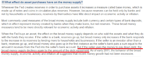
In Post-Keynesian monetary theory, economists say that the stock of money is “demand-determined” and Hetzel’s arguments seems to be against this view. However what Hetzel forgets is that while the Federal Reserve influences the stock of money, it is still demand-determined. This is because money-demand depends on agents’ portfolio preferences. If agents have “excess” stock of money, they may reflux this by reducing their loans toward the banking system – just like Post-Keynesians claim. The Federal Reserve QE Education page New York Fed 101: The Federal Reserve’s $600 Billion Treasury Purchase Program (Called by some QE or QE2) itself says so:

In fact since QE leads to higher asset prices, economic units may in fact borrow more funds to invest (read: speculate) in the stock markets.

Also note that “money-demand” is dependent on various things such as expected returns on substitutes. To the first approximation we may say that the stock of money was determined by the Federal Reserve since it has an eye on the monetary aggregates (although not targeting in the Monetarist sense). But once the process is set in motion, it then becomes endogenous because of behaviour of economic units.

Only in the limited case of settlement balances can we say that a monetary aggregate (monetary base or MB in this case) was set by the central bank.

The correct way of seeing this is via using Wynne Godley’s asset allocation model. In this what the variable M_d is still decided by household behaviour – which depends on portfolio preferences, wealth, income and expected returns on all assets. LSAP works by reducing the supply of long-term bonds and hence reducing long-term yields via the “preferred-habitat” theory and hence increasing demand for other assets via imperfect asset substitution and changing their prices.

This itself has an influence on money-demand (because money-demand also depends on expectations of returns of other assets) but the amount of asset purchases by the Fed doesn’t determine the stock of money at any point in time.

Hence Hetzel is both wrong by appealing to the money multiplier mechanism and even if he hadn’t his other point about the stock of money being supply-determined is incorrect.

You can read Nick Edmonds’ blog on how this works – he has the most precise way of describing QE/LSAP.

Eugene Fama was on CNBC today (US time) (video here) and he argued that QE is a non-event.

Since he was on CNBC, I presume he has prices of financial assets in mind when he says it is a “non-event” – the logic being that the Federal Reserve and the Treasury together have effectively issued short-term debt and reduced the supply of long term debt.

Of course while this it is true that there is reduction of the supply of long term debt and increase in short term debt (compared to the counter-factual), it doesn’t mean it has no effect whatsoever. Of course Fama says it may have minor effect and the description of QE as a non-event is just a quick way of communicating his point, even if he is true, it is not that simple.

But first, it is great to see Fama doesn’t say this has led to a rise in prices of goods and services!

The U.S. Federal Reserve has purchased long term bonds – such as US Treasury securities and agency mortgage-backed securities by settling the purchase by issuing settlement balances to banks’ accounts at the Federal Reserve (in either case when a bank or a non-bank is a buyer).

This is however different from any other operation changing the composition of the bonds held by the private sector because in QE, banks have been holding balances at the Federal Reserve which they may not have held otherwise. As a counterpart to this the money stock compared to the counter-factual is also higher. Because of this, the non-bank private sector will “re-balance” its portfolio and this will clear via a higher price of assets such as bonds and equities.

In general investors – both residents and nonresidents – are also interested in international assets and this will lead to a price rise of equities in other countries as well because of capital inflows (from their perspective). Of course, one may argue that a capital flow in one direction is compensated by an outflow in the other direction but this needn’t mean there is no effect because this “clearing” occurs via changes in prices – such as exchange rates and prices of assets in the resident issuer’s currency.

There are two effects here. Prices of financial assets may change purely because of rise in expectations and also due to a rise in demand for the asset when expectations are held constant. In general both will have an effect because these two cannot be cleanly separated.

There are some who try to argue that as if it is only the expectations that matter – as if the rise is purely due to a change in investor sentiment and not due to a change in asset demand. From the point of view of asset allocation theory however, both matter.

Another thing is how much effect a billion of “asset purchase” by the Federal Reserve has. That is a slightly different question. In modelspeak it is that depends on the various parameters of the portfolio preferences. However there are people who say this is difficult to measure empirically. True but exactly for the same reason, it is also difficult to empirically say what effect this will have when if the Federal Reserve “tapers” QE.

At any rate, the point is that saying that the large scale asset purchases of the Federal Reserve or QE is just like another debt management operation is not a good argument because in QE, banks hold the short term debt of the official sector which is not the case in ordinary debt management operations and the counterpart to this is the rise in the money stock than otherwise leading to portfolio re-balancing by the non-bank private sector and the overseas sector.

There are some who think that Tobin’s asset allocation ideas (which was what Ben Bernanke had in mind when he started QE) are incorrect. Recently emerging market currencies saw sharp depreciation when it was thought the Federal Reserve may taper. Whether this was due to incorrect sentiments or due to whether the asset allocation theory applies is another question – the Federal Reserve Open Market Committee (FOMC) still has to consider these things when taking a decision on tapering because even if the asset allocation theory on which it has based its LSAP is wrong, investor sentiment may itself can have negative effects on financial markets.

Looking at the matter more academically, the thinking that “there is no portfolio rebalance” is equivalent to thinking that money (as in deposits) are held non-volitionally by the non-bank sector – something which doesn’t sound right.

In the above I avoided arguing how much effect QE has had on asset prices because as I mention it is difficult to empirically conclude. In my opinion it is quite strong. But irrespective of this, the fact that it is difficult to know empirically (but with some data from depreciation of currencies of “emerging markets”) also means that it is difficult to say what happens if there is “taper”. You could argue that there was no effect to begin with and hence there is no trouble withdrawing it but there is a risk that you may be wrong!

Personally I think QE is a waste of time but for different reasons. It somehow misleads policy makers – the ones making fiscal decisions to wishfully think something good is going to happen. Financial markets however seem to be worried at the mere mention of “taper” so the best way for the Federal Reserve would be to convince that this is silly – slowing down is not to be worried about.

There is an article by Raj Chetty Yes, Economics Is A Science getting some attention – including that of Greg Mankiw who comments:

An interesting article, which raises the following questions in my mind: Is the younger generation of economists like Raj skipping some of the big questions of economics because some smaller questions are easier to answer?  If so, is that optimal from the standpoint of society as a whole?

There are two things here: The question whether Economics is a science hides the fact that most economists at the most basic level are simply incompetent and struggle with basic economic concepts. This can come across as pompous but you only have to look to believe it. The Mankiw quote above is another level of shamming.

In other subjects – science or in arts – if you have the talent, there is a good chance you are successful and lead a good life. Of course one can fail or not do well for various other reasons such as having a failed love relation affecting your performance and so on, but if you are interested in economics early in life and go to a university to study, ability can make your life difficult and even miserable because your professors don’t know anything.

While it is a good debate to compare Economics to sciences such as Physics, the trouble is that almost all economists at the most elementary level fail to understand the most basic things.

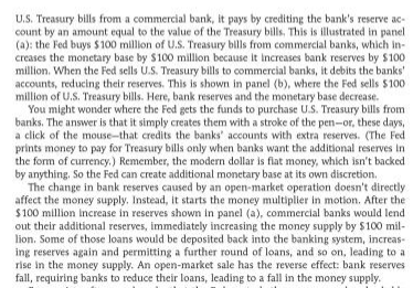
Take for example the textbook on Macroeconomics by Krugman and Wells. If you are interested even partly in Macroeconomics and skim through heteredox blogs, you will find out how the concept of the “money multiplier” is erroneous to say the least. But look at what the authors say in page 399 of the 3rd edition:

(source: amazon.com)

And this – the money multiplier story – is just one example among numerous others. The question of whether economics is science or not is sometimes irrelevant when at the most basic level, most economists failed to understand simple things.