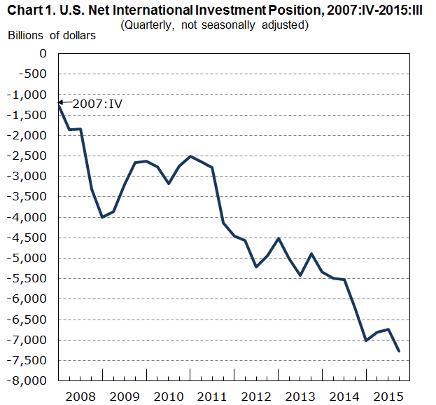
Monthly Archives: March 2016

Getting Paid To Have A Trade Deficit?

intinv315-chart-01

Source: BEA.

Eric Lonergan has written an interesting post about US trade deficits on his blog Philosphy Of Money/Sample Of One. In the post Eric claims that the United States is not a debtor of the world but that she is a creditor of the world! Eric also says that a lot of talk of all this is conventional wisdom and in reality the United States is getting paid to have lunch.

First, it’s no conventional wisdom. Most of standard macroeconomics is simply denying the importance of balance of payments. It is held that market mechanisms will correct imbalances, if only the government does its job. So there’s no conventional wisdom worrying about the trade deficit of the United States of America. It is exactly the opposite – a heterodox view.

Second, there is no “free lunch”. Imports put a drain on demand and output and because of the imbalance of the U.S. trade, full employment has been a distant dream. With so much of unemployment (especially in the crisis) and the slow recovery, one cannot claim that the U.S. has some free lunch. Only if there is full employment and that too remaining sustainable, can one claim that there’s some “free lunch”. A smaller point is that one needs the correct counter-factual: if the U.S. trade deficit had been lower, interest income (one of Eric’s main points) would have been even higher. So one more reason to avoid the phrase “free lunch”.

Moving to more important points. Eric claims that net return of FDI is high and hence BEA’s numbers are not right. Specifically he claims:

So here’s the crux: American generates a high positive net income from its net international asset position – which implies its net external asset position is a positive number. Despite running permanent current account deficits, the US has accumulated net external assets. this sounds less counterintuitive if you think that all it means is that US assets oversees are more valuable than foreign holdings of US assets.

To highlight how significant the difference is, BEA measures of US net external liabilities are around $7trn, if we simply value the net income on a PE multiple of 14x, the net external assets of the US are around $2.7trn!

An inconsistency this large seems extreme, but consider the valuation of foreign direct investment (FDI). According to the BEA, net FDI of the US has a value of less than $1trn, although the US earns $424bn on its overseas FDI and foreign FDI in the US only earns $153bn. If we value both income streams on 14x earnings, the US has net FDI assets of $4.2trn – the BEA ‘market value’ estimates are out by $3trn.

Now, that is not a correct way to approach this. To see the error, assume the stock of outward FDI is $100 and the stock of inward FDI is also $100 at market prices. Suppose investment receipts is $10 and income paid is $9. So it looks like the United States is earning $1 on a net FDI of 0. So according to this argument, the return is infinite!

It is better to look at the actual numbers:

Stocks

Outward FDI: $6,695bn

Inward FDI: $6,196 bn.

Flows

Direct investment income: $776bn

Direct investment payments $592bn.

There is nothing drastically wrong about these numbers. Perhaps, it can be argued that direct investment in the US by foreigners will take time to pay off, or that foreigners are satisfied with this or something else. These numbers do not appear wrong.

Netting inward and outward and comparing returns to the net stock is an invalid argument, as I showed above with an example of inward/outward FDI of $100.

In addition, on Twitter Eric says a DCF (discounted cash flow) model also supports his thesis that the United States is a net creditor. The loophole in this argument is that it holds assets and liabilities vis-à-vis foreigners fixed. But because the United States runs current account deficits, liabilities rise faster than assets attributable to the deficit. So even if the U.S. earns interest income, net, from abroad, this effect will catch up.

There’s other way of saying all this. If is return on assets and are assets and liabilities.

rA > rL

rA ·A > rL·L

is not inconsistent with

A < L

Second, using subscripts, 0 and 1 for now and some point in future,

rA0 ·A0 > rL0·L0

does not imply automatically that

rA1 ·A1 > rL1·L1

because liabilities can rise faster than assets (because of current account deficits) and even if return on assets is higher than return earned by foreigners on U.S. liabilities, net interest income can turn negative.

Anyway, the point of this post is that while netting is a good concept, one cannot blindly net accounting numbers. The example, a net FDI of $0 earning a net income of $1 and hence infinite return(!) is not a valid way of doing accounting. BEA’s numbers look correct.

Helicopters

Frequently, economists start discussing helicopters. This is the most counter-productive discussion. There are two things due to which they invoke this:

  1. Confusion
  2. Intent

The confusion part is basically due to economists’ complete failure to understand what money is and how to account for it and this is due to a lack of training in national accounting/flow of funds etc.

The intent part is equally important. This is because economists are trained in thinking of fiscal policy as impotent. After the crisis, they have party understood the role of fiscal policy but the notion that fiscal policy is impotent is so deeply ingrained that it’s difficult for them to come out of it. This reason is not so obvious but can be proved as follows: If they really think that fiscal policy is not impotent, they should rather suggest a rise in government expenditure than some helicopters.

There’s a third reason.

Wynne Godley in his paper Money, Finance And National Income DeterminationJune 1996 had a good description of all this:

Modern textbooks on macroeconomics treat money in a remarkably uniform – and remarkably silly – way. In the primary exposition the stock of “money” is treated as exogenous in the two senses a) that it is determined outside the model and b) that it has no accounting relationship with any other variable. The reader is then invited to assume, pro tem, that the central bank controls “the money supply” so that it is constant through time. When the operations of banks are described, typically some thirty chapters later, the quantity of money is some multiple of commercial banks’ reserves as a consequence of these institutions having become “loaned up”.

Silly? The money stock, as revealed in real life financial statistics, is as volatile as Tinkerbell – for good reasons, as I shall argue below. How can it be sensible to undertake a thought experiment in which the flickering quantity called “money” is literally constant through periods at least long enough for capital equipment to be planned, built and commissioned – and for lots of other things to happen as well? And the other, “money multiplier”, story has the strange defect that, while giving some account of how credit money might be created, it completely ignores the impact on spending of the counterpart changes in bank loans which are assumed to be taking place; perhaps it is because loan expenditure would mess up the solution of the IS-LM model when alternative assumptions about “the money supply” are used, that the supposed process of money creation normally gets separated from that of income determination by so many chapters.

The bibles of the neo-classical synthesis don’t help. There is a spectacular lacuna in the constructions presented, for instance, by Patinkin, Samuelson and Modigliani with regard to the asset side of commercial banks’ balance sheets. Usually the role and
even existence of bank credit is simply ignored. Modigliani (1963) gives banks (with regard to their assets) no role other than to hold government bonds; and Milton Friedman famously used a helicopter when he wanted to get more money into the system.

There is a reason for all this. It is that mainstream macroeconomics postulates in its basic model that macroeconomic outcomes are all determined by relative prices established in Walrasian markets. Individual agents are held to engage in a market process of which the outcome is to find prices for product, labour and money which clear all three markets plus, by Walras’s law, the market for “bonds”. But as is now well known, there is no use for money in the Walrasian world even though, paradoxically, “money” is a logical necessity if the model is to be solved.

[boldening: mine]

There is no need for helicopters. All is needed is a description via social accounting (i.e. national accounting). Just say “increase government expenditure” to the government or “expand fiscal policy”.

Link

What Post-Keynesian Economics Has Brought To An Understanding Of The Global Financial Crisis

I came across a nice Marc Lavoie paper from July 2015 from which I borrowed the titled of this post. Marc Lavoie discusses the importance of PKE monetary economics, stressing flow-of-funds modelling such as as done by Wynne Godley and his prescient analysis of the fate of the US economy and the rest of the world.

(the post title is the link)

Robert Blecker has a great article from the same conference (annual conference of the Canadian Economics Association) discussing similar things: heteredox understanding of the crisis. He discusseses Wynne Godley’s Seven Unsustainable Processes. He also talks of Hyman Minsky and neo-Kaleckian models of how income distribution effects aggregate demand. His paper titled Finance Distribution And The Role Of Government: Heterodox Foundations For Understanding The Crisis is here.

Is Floating Better? Is The Stock Of Money Exogenous In Fixed Exchange Rate Regimes?

I believe that the basic problem today is not the exchange rate regime, whether fixed or floating. Debate on the regime evades and obscures the essential problem … Clearly flexible rates have not been the panacea which their more extravagant advocates had hoped … I still think that floating rates are an improvement on the Bretton Woods system. I do contend that the major problems we are now experiencing will continue unless something else is done too.

– James Tobin, A Proposal For Monetary Reform, 1978

Frances Coppola has written a post saying that floating exchange rates are not the panacea. Although I agree with her point, there are however a few points in her article which has some issues. She says that money stock is exogenous in gold standard.

Under a strict gold standard, the quantity of money circulating in the economy is effectively set externally. The domestic money supply can only grow through foreign earnings, which bring gold into the country.

… This is evident from the quantity theory of money equation MV = PQ, which is fundamentally flawed in a fiat currency fractional reserve system but works admirably under a strict gold standard or equivalent.

Frances is critiquing Neochartalists there but ends up accepting their notion that macroeconomics is something different when a nation’s currency is not floating and there’s an exogenous stock of money in fixed exchange rate regimes. There is absolutely no proof that it is so. Money stock can grow if there’s higher economic activity due to rise in private expenditure relative to income or via fiscal policy. But why this obsession with Monetarism? It doesn’t work anywhere: whether the exchange rate is fixed or floating. All arguments made in Post Keynesian economics carry through to the gold standard. Indeed Robert Mundell himself realized this in 1961 [1].

Here’s a quote from the book Monetary Economics by Wynne Godley and Marc Lavoie, page 197, footnote 11:

It must be pointed out that Mundell (1961), whose other works are often invoked to justify the elevance of the rules of the game in textbooks and the IS/LM/BP model, was himself aware that the automaticity of the rules of the game relied on a particular behaviour of the central bank. Indeed he lamented the fact that modern central banks were following the banking principle instead of the bullionist principle, and hence adjusting ‘the domestic supply of notes to accord with the needs of trade’ (1961: 153), which is another way to say that the money supply was endogenous and that central banks were concerned with maintaining the targeted interest rates. This was in 1961!

Bretton Woods was the emperor’s new clothes and floating exchange rates are the emperor’s new new clothes. The important question is whether floating exchange rates offer any market mechanism to resolve balance of payments imbalances and the answer is that it doesn’t. In gold standard, current account deficits can be financed by official sale of gold in international markets and residents borrowing from abroad. In floating exchange rate regimes, it is financed by borrowing from abroad. Hardly much difference. So the main adjustment is left to movement of the exchange rate. One needs to suspend all doubt and believe in the invisible hand to think the movement of exchange rates can do the trick. The reason it is the emperor’s new new clothes is that the promises never worked. And similar promises were made by economists that there’s a market mechanism to resolve balance of payments imbalances in fixed exchange rate regimes.

To summarize, my argument is that the only point to debate is whether floating the exchange rate resolves imbalances as compared to fixed exchange rates, not about the endogeneity of money. Although there is a role because of the movement of the exchange rate, floating exchanges is not a panacea. Although I am not on the side of the Neochartalists in the debate, I thought I’d point this out: do not fall into the pitfall of your opponent.

  1. Mundell, R. (1961) ‘The international disequilibrium system’, Kyklos, 14 (2),
    pp. 153–72.

The ‘Paradox’ Of Protectionism

Paul Krugman says trade wars are a wash. Brad Delong is raising his neoliberal freak flag high.

Who is right? Answer: Neither. Global output will rise under non-selective protectionism (or has an expansionary bias, to be more precise). Protectionism reduces the propensity to import. That doesn’t mean imports will fall. Total imports of an individual nation will rise because of higher income. World trade will rise because of higher world income.

In other words, non-selective protectionism acts by reducing the propensity to import by price elasticity effects but raises volume of imports via income elasticity effects.

The world as a whole is balance-of-payments constrained, not just individual nations. Raising tariffs on imports incentivises producers to produce more as they will face less competition from abroad. Consumers will shift to domestically produced goods because of price elasticity effects.

Moreover, since governments of most nations won’t have a balance-of-payments constraint if there are large tariffs, they will be free to boost domestic demand by fiscal policy, limited only by the economy’s capacity to produce. If it is done, it will be a conscious behaviour by the government.

There is of course another way fiscal policy gets relaxed because of balance of payments. Reduction of current account deficits, relative to gdp, reduces the budget deficit, relative to gdp (as can be shown by a behavioural model and this shouldn’t be surprising as the two are related by an accounting identity). Typically governments follow some rules even if they aren’t explicitly required and their expenditure is endogenous to the government budget deficit: they tighten fiscal policy when the budget deficit goes out of a limit and relax fiscal policy when the budget deficit is within the limit. So improvement in a country’s balance of payments position would lead to a relaxation of fiscal policy, automatically.

To summarize, protectionism if done the right way can raise world trade because of rise in world income. There is no economic case against protectionism. There is opposition because few corporations want to increase their share in world markets. Protectionism reduces share of these mega corporations instead of reducing world trade. So “free trade” (which is managed trade for a few) only benefits a few and imposes a huge cost on the world economy.

All that is for the current world economic outlook. Typically in deep recessions governments take protectionist measures. In such scenarios, since output is falling, there is a tendency to confuse this with causation. It is more accurate to say that protectionism prevented a deeper implosion in such cases.

Non-selective Protectionism In Wynne Godley’s 1999 Article Seven Unsustainable Processes

‘Free Trade Loses Political Favour,’ says the front-page of today’s Wall Street Journal.

Free Trade Loses Political Favour

Paul Krugman has two articles conceding that he held wrong views earlier.

Krugman says:

But it’s also true that much of the elite defense of globalization is basically dishonest: false claims of inevitability, scare tactics (protectionism causes depressions!), vastly exaggerated claims for the benefits of trade liberalization and the costs of protection, hand-waving away the large distributional effects that are what standard models actually predict.

Krugman claims that he hasn’t done any of it but a reading of his 1996 article Ricardo’s Difficult Idea says the exact opposite.

The earliest cri de cœur of the U.S. balance of payments situation came from Wynne Godley in his 1999 article Seven Unsustainable Processes. 

In his sub-heading ‘Policy Considerations,’ he says:

Policy Considerations

The main conclusion of this paper is that if, as seems likely, the United States enters an era of stagnation in the first decade of the new millennium, it will become necessary both to relax the fiscal stance and to increase exports relative to imports. According to the models deployed, there is no great technical difficulty about carrying out such a program except that it will be difficult to get the timing right. For instance, it would be quite wrong to relax fiscal policy immediately, just as the credit boom reaches its peak. As stated in the introduction, this paper does not argue in favor of fiscal fine-tuning; its central contention is rather that the whole stance of fiscal policy is wrong in that it is much too restrictive to be consistent with full employment in the long run. A more formidable obstacle to the implementation of a wholesale relaxation of fiscal policy at any stage resides in the fact that this would run slap contrary to the powerfully entrenched, political culture of the present time.

The logic of this analysis is that, over the coming five to ten years, it will be necessary not only to bring about a substantial relaxation in the fiscal stance but also to ensure, by one means or another, that there is a structural improvement in the United States’s balance of payments. It is not legitimate to assume that the external deficit will at some stage automatically correct itself; too many countries in the past have found themselves trapped by exploding overseas indebtedness that had eventually to be corrected by force majeure for this to be tenable.

There are, in principle, four ways in which the net export demand can be increased: (1) by depreciating the currency, (2) by deflating the economy to the point at which imports are reduced to the level of exports, (3) by getting other countries to expand their economies by fiscal or other means, and (4) by adopting “Article 12 control” of imports, so called after Article 12 of the GATT (General Agreement on Tariffs and Trade), which was creatively adjusted when the World Trade Organization came into existence specifically to allow nondiscriminatory import controls to protect a country’s foreign exchange reserves. This list of remedies for the external deficit does not include protection as commonly understood, namely, the selective use of tariffs or other discriminatory measures to assist particular industries and firms that are suffering from relative decline. This kind of protectionism is not included because, apart from other fundamental objections, it would not do the trick. Of the four alternatives, we rule out the second–progressive deflation and resulting high unemployment–on moral grounds. Serious difficulties attend the adoption of any of the remaining three remedies, but none of them can be ruled out categorically.

[italics in original, underlying mine]

Link

Flow Of Funds Sankey Diagrams

The UK ONS (Office of National Statistics) has launched a new set of statistics: the flow of funds for the UK economy.

The recent financial crisis re-emphasised the importance of monitoring the build-up of financial risks in the economy. Since then, there have been renewed calls for identifying balance sheet exposures between different institutional sectors.

Building on recently published flow of funds experimental statistics by Office for National Statistics, in partnership with the Bank of England, this article takes a further step in exploring sectoral interconnectedness within the UK economy and analyses these lender-borrower relationships in the context of risk exposures. Using data visualisation techniques, we illustrate how financial counterparty relationships have changed over time and infer what this tells us about the transmission of financial risks.

In addition, there is an interactive Sankey diagram on the site.

Fun!

(The title of this post is the link).

UK Flow Of Funds Sankey Diagram

Bernie Sanders, U.S. Private Sector Deficits And Balance Of Payments

Over his blog The Beauty Contest – A blog on Spanish and international affairs, macroeconomics and finance, Javier López Bernardo has an analysis of Bernie Sanders’ economic plan (written with his colleague Rafael Wildauer).

Javier López Bernardo and  Rafael Wildauer stress the importance of the U.S. balance of payments constraint on U.S. growth. He uses a sectoral financial balances model to highlight how sectoral balances would look under Bernie Sanders’ plan: an exploding combination of U.S. private debt and negative net international investment position because of exploding negative financial balance of the private sector and the U.S. economy as a whole.

Also, they say:

We have not intended to bash Mr. Sanders’ economic program (actually, we are quite sympathetic with most of its measures) or Prof. Friedman’s economic exercise (which is useful to frame the economic discussion), but simply to highlight the incompleteness of economic analysis carried out in closed-economy frameworks – as the critics and Prof. Friedman’s exercise have exemplified.

Their projection is this chart:

Sanders-projection-KFBM

Discrete Time Or Continuous Time?

There is always some debate by people on how continuous time is better modelling. A James Tobin quote from his Nobel Lecture comes to mind.

Macroeconomic Modeling Strategy: Continuous or Discrete Time

The issues just discussed are related to the modeling of time. The equations introduced above count time in discrete periods of equal finite length. Within any period, each variable assumes one and only one value. In particular, clearing of asset markets determines one set of asset prices per period. From one period to the next asset stocks jump by finite amounts. Therefore the demands and supplies for these jumps affect asset prices and other variables within the period, the more so the greater the length of the period. They will also, of course, influence the solutions in subsequent periods.

The same modeling strategy can be used with continuous time. The specific saving functions, as well as the total saving function, then tell the rate at which savers want to be increasing their stocks of particular assets and of total wealth. They will reflect both the continuous execution of long run saving and portfolio plans and the speeds of adjustment of stocks to deviations from these plans that arise because of surprises, news, and altered circumstances or preferences.

Either representation of time in economic dynamics is an unrealistic abstraction. We know by common observation that some variables, notably prices in organized markets, move virtually continuously. Others remain fixed for periods of varying length. Some decisions by economic agents are reconsidered daily or hourly, while others are reviewed at intervals of a year or longer except when extraordinary events compel revisions. It would be desirable in principle to allow for differences among variables in frequencies of change and even to make those frequencies endogenous. But at present models of such realism seem beyond the power of our analytic tools. Moreover, many statistical data are available only for arbitrary finite periods.

Representation of economies as systems of simultaneous equations always strains credibility. But it takes extraordinary suspension of disbelief to imagine that the economy solves and re-solves such systems every microsecond. Even with modern computers the task of the Walrasian Auctioneer, and of the market participants who provide demand and supply schedules, would be impossible. Economic interdependence is the feature of economic life and we as professional economists seek to understand and explain. Simultaneous equations systems are a convenient representation of interdependence, but it is more persuasive to think of the economic processes that solve them as taking time than as working instantaneously.

In any event, a model of short-run determination of macroeconomic activity must be regarded as referring to a slice of time, whether thick or paper thin, and as embedded in a dynamic process in which flows alter stocks, which in turn condition subsequent flows.

Subscripting Helps!

The accounting identities equating aggregate expenditures to production and of both to incomes at market prices are inescapable, no matter which variety of Keynesian or classical economics you espouse. I tell students that respect for identities is the first piece of wisdom that distinguishes economists from others who expiate on economics. The second? … Identities say nothing about causation.

– James Tobin, 1997, p. 300, ‘Comment’, in B.D. Bernheim and J.B. Shoven (eds), National Saving and Economic Performance, Chicago: University of Chicago Press.

This is a continuation of my post Stock-Flow Inconsistent? which was a reply to Jason Smith’s blog post More like stock-flow inconsistent on his blog Information Transfer Economics. If you had checked my post before around noon UTC yesterday, you might want to check the updated version.

Jason Smith also has updated his post and proposes a new equation:

ΔH = Γ·(G – T)

(incorrect equation)

Now, that’s quite wrong because it violates rules of accounting.

Morever, Jason Smith insists that it is a behavioral equation.

A lot of clarity can be achieved if one uses subscripts, so that things are clearer.

So we have two equations:

ΔH = GT

dH/dt = GT

Although these two are related, they are not exactly the same: the former is in a difference equation form and the latter in the differential equation form. The in the former has no time dimensions and the in the latter has time dimension equal to –1. The in the former is total expenditure in a period, the in the latter is a rate. 

Since stock-flow consistent models are written typically in difference equations, rather than differential equations, let us avoid subscripts for difference equations for the former and use it for latter.

So it is better to write the equations as:

ΔH = G – T

dHcontinuous/dt = Gcontinuous – Tcontinuous

Each time step in the formalism of difference equations is Δt and hence

G = Gcontinuous ·Δt

T = Tcontinuous ·Δt

Hcontinuous = H

So,

ΔHt = Gcontinuous – Tcontinuous

(approximately)

Or,

ΔH/ Δt = Gt – Tt

Or,

ΔH = G – T

So instead of reaching the correct equation which is:

ΔH= Δt · (Gcontinuous – Tcontinuous)

Jason reaches the equation:

ΔH = Γ·(G – T)

(incorrect equation)

But

ΔH = G – T

as it is an accounting identity in the model!